SACHIN S. BHARADWAJ¹ and KATEPALLI R. SREENIVASAN^1,2,3,4*
¹ Department of Mechanical and Aerospace Engineering, New York University, New York 11201 USA
² Department of Physics, New York University, New York 10012 USA
³ Courant Institute of Mathematical Sciences, New York University, New York 10012 USA
⁴ New York University, Abu Dhabi 129188, UAE

^*Corresponding author. E-mail: katepalli.sreenivasan@nyu.edu

MS received 15 2020; revised 15 2020; accepted 15 2020

Abstract. . . .

Keywords. .

PACS Nos 12.60.Jv; 12.10.Dm; 98.80.Cq; 11.30.Hv

. . . (HPC) (DNS) . . . . !

. “”. Richard Feynman [1] . NISQ (Noisy Intermediate Scale Quantum) [2] 50 . ( .) “” . (QC) . . (CFD).

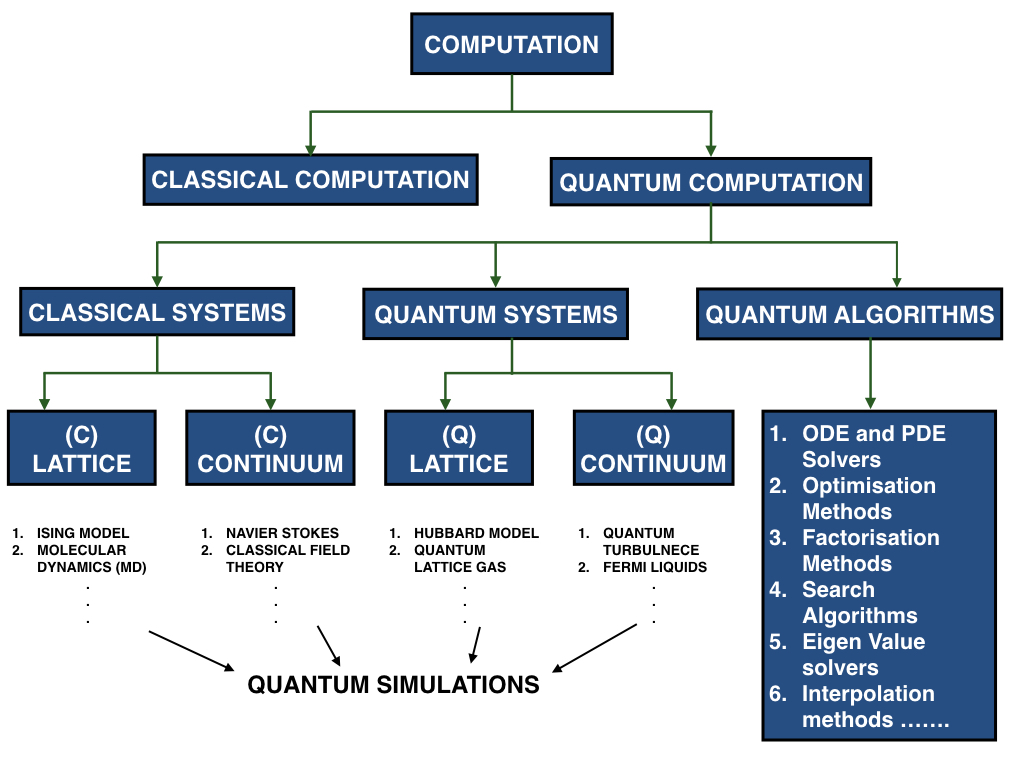
CFD (QCFD). . 2 QC . 3 QC. ( 4) ( 5). 5 . 6 QC . 7 QCFD 7.

QC . [3].

2.1

“” “ ” “ ” . “”. .

Figure 1. . α β γ

2.2

. . . Ψ . . (QED) Rydberg ( Majorana) (NMR) . . Hilbert ℍ. bra-ket Dirac “ket” |Ψ⟩ ℍ (∈ ℂⁿ)

⌊ ⌋ ||||c1|||| |ψ⟩ =|||||c2|||||;c ∈ ℂ ||||| ...||||| i ⌈cn⌉

(1)

“bra” ⟨Ψ| = |Ψ⟩^†. . Hilbert : |Ψ⟩ = (|ψ₁⟩⊗... ⊗|ψ_n⟩) ∈ ℍ^⊗n. ( ↑ ↓) |0⟩|1⟩ . ℍ ∈ ℂ^⊗2

|Ψ ⟩ = c1|0⟩+ c2|1 ⟩,

(2)

[ ] [ ] 1 0 |0⟩ = 0 and |1⟩ = 1 .

(3)

Figure 2. NOT

Figure 3. NOT

Figure 4. NOT

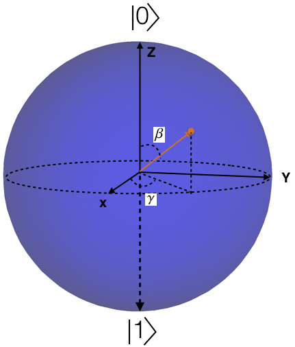
c₁ c₂ |c₁|² |c₂|² Born |0⟩ |1⟩. . ( .) : . . Hilbert Bloch 1. (2)

[ (β) (β) ] |Ψ⟩ = eiα cos--|0⟩ + eiγsin --|1⟩ , 2 2

(4)

α γ ( ) β . “ ” Bloch.

Table 1.


Quantum Logic Gate	Circuit Symbol	Operation



X(Pauli X)	$X$	\|0⟩ → \|1⟩ \|1⟩ → \|0⟩

Y(Pauli Y)	$Y$	\|0⟩ → i\|1⟩ \|1⟩ → −i\|0⟩

Z(Pauli Z)	$Z$	\|0⟩ → \|0⟩ \|1⟩ → −\|1⟩

H(Hadamard)	$H$	\|0⟩ → $\|0⟩+√\|1⟩- 2$ \|1⟩ → $\|0⟩−√\|1⟩ 2$

R_ϕ(Phase Shift)	$T$	\|0⟩ → \|0⟩ \|1⟩ → e^iϕ\|1⟩


CNOT	$\|q\|q12⟩⟩$	\|q₁,q₂⟩ → \|q₁,q₂ ⊕q₁⟩

SWAP	$\|\|qq1⟩2⟩$	\|q₁,q₂⟩ → \|q₂,q₁⟩

To↑oli	$\|q\|q\|q ⟩⟩⟩ 123$	\|q₁,q₂,q₃⟩ → \|q₁,q₂,q₃ ⊕q₁ ⋅q₂⟩

2.3

AND NOT OR NAND To↑oli .

U (UU^† = 𝕀) . ( NOT) . 1. [3].

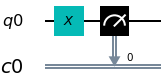
. NOT . X σ_x Pauli. (q0) |ψ⟩ = $√--- 0.6$ |0⟩+ $√--- 0.4$ |1⟩
X = σ_x = $[ ] 0 1 1 0$ .

[0 1][1] [0] [0 1 ][0] [1 ] = and = . 1 0 0 1 1 0 1 0

(5)

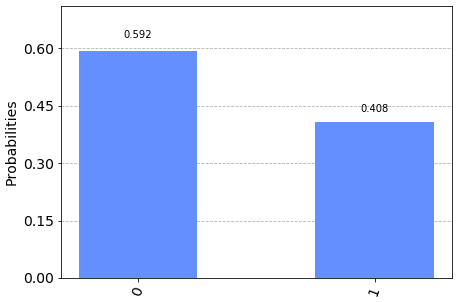
|0⟩ → |1⟩|1⟩ → |0⟩. (|c₁|² |c₂|²) (c0) 2. . X NOT .

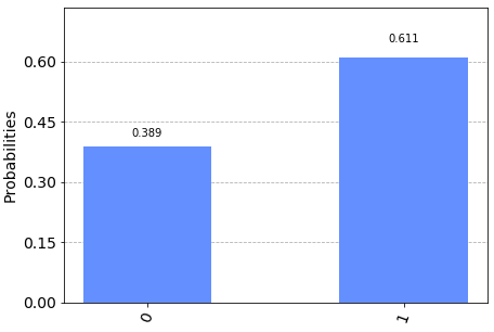
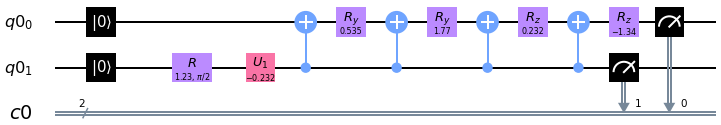
IBMQ Qiskit 3 4 . NOT |0⟩|1⟩ |ψ′⟩ = $√0.4-$ |0⟩+ $√0.6-$ |1⟩. . .

2.4

Figure 5.

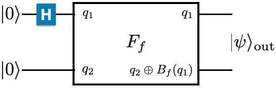
B_f: {0,1} $↦→$ {0,1}. 0 1 . 2 |ψ_in⟩ = |q₁q₂⟩ q₁,q₂ ∈ {0,1}. ( ) F_f |q_1,q₂⟩ $Ff −−→$ |q₁,q₂ ⊕ B_f(q₁)⟩ ⊕ 2 ( [3] ). B_f(0) B_f(1) . 5 : Hadamard : |0⟩⊗|0⟩ $H−−−⊗→𝕀$ $|0⟩+√|1⟩- 2$ ⊗|0⟩. F_f

|0,B f(0)⟩+ |1,Bf(1)⟩ |Ψ ⟩out =--------√---------. 2

(6)

Figure 6. QC

B_f(0) B_f(1). . B_f Deustch-Josza Simon [3]. QC QC . .

3. :

: . QC 6 . QC: (1) (2) (3) . .

3.1

QC. :

(a) : Hubbard . Hamiltonian .

(b) : Schrödinger . Gross Pitaevski ( ) Monte Carlo .

3.2

. . . Boltzmann ODE Navier-Stokes.

3.3

. ODE/PDE .

. : (1) (2) .

(DNS) [4, 5, 6, 7, 8] (LES) [9, 10, 6] Navier-Stokes Reynolds (RANS) [6, 11] Boltzmann (LBM) [12, 13] . LBM Boltzmann “ ” . - 7. . LBM

(∂t + vα.∇)ρα(r,t) = Sαβ(ρeq(r,t)− ρβ(r,t)). ◟-----------------◝◜ -----------------◞ ◟----------β-------------◝◜-----------------------◞ Advection Scattering-Relaxation

(7)

v ρ S ρ^eq ( [13]). “” ( ) QC .

Figure 7. LBM

4.1 LQC 1:

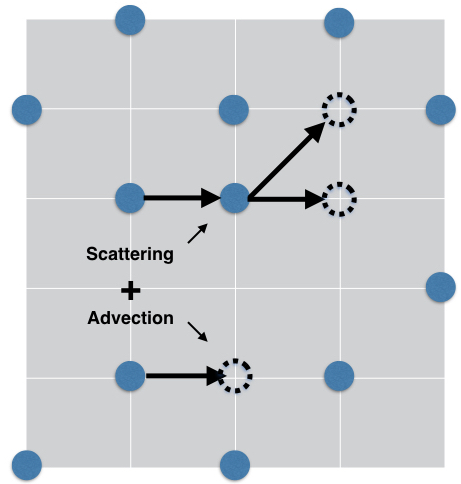
QC. QC ( QC ) QCs . (QLGA) [14, 15] .

1D. (x,v)_i v_i . 1D . LBM 7 .

QLGA . 1D N 2 (q) (l) (r) . 2 |ψ⟩_i = α|q₁q₂⟩_i + β|q₁q₂⟩_i q₁,q₂ ∈ {l,r} {|lr⟩,|ll⟩,|rr⟩,|rl⟩}. Ŝ Â. L R ( ) ( p)

( ) ( ) S = L R = cos p isin p 1 R L isin p cos p

(8)

( ) ( ) ||||1 0 0 0|||| ||||1 0 0 0|||| S2 = ||||0 L R 0||||= ||||0 cos p isin p 0||||, |||(0 R L 0|||) |||(0 isin p cos p 0|||) 0 0 0 𝜃 0 0 0 𝜃

(9)

|L|² + |R|² = 1 = |𝜃|² 𝜃 . :

Ψ(r,t + 1; →)	= LΨ(r −1,t; →) + RΨ(r + 1,t; ←)	(10)
Ψ(r,t + 1; ←)	= LΨ(r + 1,t; ←) + RΨ(r −1,t; →).	(11)

L R p . Schrödinger. Dirac Schrödinger δr → 0 δr² → 0 δt → 0 Chapman-Enskog [14, 16, 17].

. QLGA [16, 17, 18, 19, 20] Burgers [21, 22, 23, 24].

. LBM . 4 4 2⁴ . QC 4 QCs . N N_q ( ) QC N_T = N ∗N_q . Hilbert 2^N_T 2^N_q Hilbert C q_i

Ψ(r₁,..,r_N,t)	= ∑ _{ψ(r_i,t)}C ×(ψ(r₁,t) ⊗.... ⊗ψ(r_N,t))	(12)
	= ∑ _{ψ_{q_i}} $˜ C$ ×(ψ_q₁ ⊗.... ⊗ψ_{q_{N_T}}).	(13)

Schrödinger (Â) (Ŝ)

Ψ(r,t + Δt) = eiHˆΔt∕ℏΨ(r,t) = AˆSˆΨ(r,t).

(14)

: Bravais R r Bloch ( k_i ≤ N ∗(period)). [22] .

(a) $nˆ$ _R = ĉ_R^†ĉ_R. QCs NMR-QC ( ) ( ).

PR,t = Tr[(|Ψ(R, t)⟩⟨Ψ(R, t)|)nˆR] = Tr[ρ(t)ˆnR].

(15)

(b) d (ξ ξv)

ξ(r,t)	= lim _d→0 ∑ _{k_i,R₁}^R_NmTr[ρ(t) $nˆ$ _{R_{k_i}}],	(16)
ξ(r,t)v(r,t)	= lim _d→0 ∑ _{k_i,R₁}^R_Nmv²r_{(RmodN_q)}Tr[ρ(t) $ˆn$ _{R_{k_i}}].	(17)

( ) .

PR+dr,t+Δt = PR,t + ⟨Ψ(R,t)|ˆS†nˆR ˆS − ˆnR |Ψ(R, t)⟩,

(18)

⟨Ψ(R, t)|ˆS†ˆn Aˆ†|Ψ(R,t+Δt)⟩ = ⟨Ψ(R, t)|Sˆ†ˆn ˆA|Ψ(R,t)⟩. R R

U₃ (IBMQ) 3 Euler [22, 25]:

( ) U = cos(𝜃2) e−iλ sin(𝜃2) . 3 eiϕsin(𝜃2) ei(ϕ+λ)cos(𝜃2)

(19)

0 ≤ (ϕ,λ) < 2π 0 ≤ 𝜃 ≤ π. : (1) LBM QC (2) (3) LBM LBM . .

4.2 LQC 2: Dirac

Figure 8. 4

LBM Dirac [12, 26, 27]. . QC QC . (7) “ Dirac Majorana” [28]

∂Ψ i-∂t + iˆApb∇pbΨ = M Ψ,

(20)

( iΔt π ( )) e−iˆAΔt∕ℏ = exp −-----√--Z1 ⊗ I2 +X1 ⊗ σpb2 . ℏ 2 2

(21)

Z_i X_i Pauli i^th σ^pb . Ŝ “ ” ( [27] ) Ŝ e^{−iŜΔt∕ℏ} = e^{Û₁+αÛ₂}. Lie-Trotter-Suzuki U₃. . . - [27]. QC QCs .

4.3 LQC 3:

d- (d+1)- . Monte-Carlo [29, 30] - [31, 32] . LQC 1 LQC2 .

Tr(e^−Hβ) Feynman

∑ Z = ⟨r|e−HΔβ∕N|r1⟩⟨r1|...|rN⟩⟨rN|e−HΔβ∕N|r⟩, r,ri

(22)

(d+1)- . 2D 1D . ( d →d [33].) . .

( ) . .

. : (1) (2) (3) . QC. .

5.1

ODE/PDE . C++ int a = 10; a 10. . QC 10 a. . . :

(1) : [34, 3] . . 1 [35] QCs ( IBMQ) . 0 0. (i) (2 + i) $√ -- 2$ i 1 ( ). N log ₂N 2 :

1( √-- ) |Ψ⟩ = --i|00⟩+ (2 + i)|01⟩ + 2i|10⟩ +1 |11⟩ . 3

(23)

1 [35] 8. ( $19$ , $59$ , $29$ and $19$ ). ( ) Qiskit— IBM Quantum Experience— 9 .

Figure 9. :

: c₁,c₂ $⋅⋅⋅$ c_n

: U_load , |Ψ⟩_{f inal} = c₁|00...0⟩+ c₂|00...1⟩+ ...+ c_n|11...1⟩

(U_zy)_i ← U_y ⊗U_z

U ← (U_zy)_i ⊗U

U = (U_zy)_n ⊗ $⋅⋅⋅$ ⊗(U_zy)₁

U_load = U^†

|Ψ_{f inal}⟩ = U_load|Ψ_{f inal}⟩ = c₁|00...0⟩+ c₂|00...1⟩+ ... + c_n|11...1⟩

return U_load, |Ψ_{f inal}⟩

DISENTANGLE(|Ψ⟩_temp):

|Ψ⟩_local = |Ψ⟩_temp ← c₁|00...q₁⟩+ c₂|00...q₂⟩+ ... + c_n|11...q_n⟩

return |Ψ⟩_local ← c₁|00...⟩⊗|q₁⟩+ c₂|00...⟩⊗|q₂⟩+ ... + c_n|11...⟩⊗|q_n⟩

Figure 10. IBMQ

Figure 11. 4

Figure 12. 3

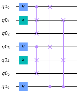
(2) : ket . 10 1010. |ψ⟩ = |ϕ⟩⊗(|1⟩+ |0⟩+ |1⟩+ |0⟩). 4 |ψ⟩ = (|0⟩|0⟩⊗|1⟩+ |0⟩|1⟩⊗|0⟩+ |1⟩|0⟩⊗|1⟩+ |1⟩|1⟩⊗|0⟩) 1010. Controlled-SWAP X H To↑oli 10. ( [36].)

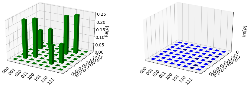
11 ρ = ∑_ip_i|ψ⟩_i⟨ψ|_i . 11 1010 . 6 4 . (N) log ₂(N) . .

5.2

. . [3, 37, 38, 39].

. . von Neumann z |0⟩|1⟩. . .

( ). .

QM: A ψ_i “a” :

“a”

$P(a) = ⟨ψi|A†aAa|ψi⟩.$ (24)
$---Aa-|ψi⟩---- |ψ f⟩ = ∘ ----†------. ⟨ψi|AaAa|ψi⟩$ (25)

“a” |ψ⟩. “” . . {|ψ_i⟩}.

. . . p_α {|ψ_α⟩} ρ = ∑_αp_α|ψ_α⟩⟨ψ_α|. ρ

“a”

$P(a) = Tr(A†aAaρ).$ (26)
$---AaρA†a--- ρ f = ∘----†----. Tr(AaAaρ)$ (27)

Tr(ρ) = 1 ( ) . : POVM (Positive Operator Valued Measure). POVM {P_{V M}^a} ≡ {A_a^†A_a} ⟨ψ_i|P_{V M}^a|ψ_i⟩ = ⟨ψ_i|A_a^†A_a|ψ_i⟩ = P(a) ≥ 0 ∑ _a P_{V M}^a = ∑_aA_a^†A_a = 𝕀. POVM $∘Pa-- VM$ = A_a.

. POVM . POVM {P_{V M}^a, P_{V M}^b and (P_{V M}^c = 𝕀−(P_{V M}^a + P_{V M}^b))} . . . . . .

5.3

. . . POVM . {𝕀∕2 X/2 Y/2 Z/2 }

ρ = 1(Tr(ρ)𝕀+ Tr(Xρ)X +Tr(Yρ)Y + Tr(Z ρ)Z ). 2

(28)

Tr(Xρ). . . 1∕ $√ -- N$ N Gaussian N . . . [40]

Bayesian.

Table 2.


#	Algorithm	Description/Used in	Complexity/Speed-up

1	Quantum Teleportation &	Inter-circuit data communication &	-
	Entanglement [3]	a fundamental block of many algorithms

2	Superdense Coding [3]	Data compression & communication	Compression Ratio 2:1

3	Quantum Fourier Transform	DFT, Phase Estimation, Period Finding,	Q: [Θ(n²),Θ(n log n)]
	(QFT) [3]	Arithmetic, Discrete log & spectral methods	C: Θ(n2ⁿ) (n=#gates)

4	Quantum Phase Estimation [3]	Quantum phases, Order Finding, Shor’s	O(t²) operations**
		Algorithm, HHL, Amplitude Amplification	t = n + $⌈ ( 1-)⌉ log 2+ 2𝜖$
		& Quantum Counting [41]

5	Grover’s Search [3, 42] &	Data search, Amplitude Estimation, Function	Q: O( $-- √ N$ )
	Amplitude Amplification [43]	minima, approx. & Quantum counting	C: O(N) (N=#ops)

6	Matrix Product Verification [44]	Verifies AB=C? (n×n matrices)	Q: ≤O(n^5∕3)); C: O(n²)

7	Quantum Simulation [19, 3]	Integrates Schrödinger equation, HHL,	superpoly
		All Hamiltonian system simulations $($ e^−iHt∕ℏ $)$	poly(n,t): n=dof, t= time

8	Gradients [45, 46]	Computes gradients, convex optimisation	quadratic - superpoly
		volume estimation, minimising quadratic forms

9	Partition Function [46] &	Evaluate/approx partition functions	quadratic - superpoly
	Sampling	Pott’s, Ising Models & Gibbs sampling

10	Linear Systems &	Solves AX=b for eigen values & vectors	superpoly - exponential
	HHL Algorithm [47, 46]	ODEs, PDEs, simultaneous eqns.
		Optimisation, Finite Element Methods etc

11	ODE [48, 46]	Integrates $˙x$ = α(t)(x) + β(t) & similar forms	superpoly - exponential

12	Wave Equation [49]	Integrates $¨ϕ$ = c²∇²ϕ & similar forms	superpoly - exponential

13	PDE / Poisson Equation [50, 51, 46]	Integrates −∇²ϕ(x) = b(x) and	superpoly - exponential
		PDEs of similar forms: Dϕ(x) = b(x)

14	QFT Arithmetic [52]	QFT based: + , - , * , mean , weighted sum	superpoly - exponential

15	Function Evaluation [53]	(Ex) inverse, exponentiation.. etc	varies
		for State Loaded data

16	VQE and QAOA [25]	Computes optimisation type problems	varies

17	Quantum Annealing [54]	Computes optimization type problems	varies

Q/C-/ VQE- QAOA-
** t = n 𝜖.

[46, 25, 40, 55]

[40]. [56]. . Bell

1 |ψ⟩ =-√--(|00⟩+ |11⟩). 2

(29)

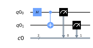
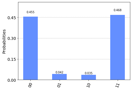
( 12) IBMQ. 1/2 . 13 (≈ 0.5) |00⟩|11⟩. . .

Figure 13.

Figure 14.

5.4

. [46, 40, 3, 25, 55]. 2 . Stokes 1D ( )

	∇²u(x) = ∇p(x)	(30)
	∇⋅u(x) = 0,	(31)

A - : u(x) . .

B - : :

: FEM . . Poisson. #13 . FEM #10 (HHL) = Alg #3 + Alg #4 + Alg #7. . [50].
: #3 (QFT) HHL . .
: # 5 .

C - : .

. Navier-Stokes. DNS FFTW . - FFTW QFT . QFT .

5.5 Fourier

Fourier [3] Fourier FFTW . . DFT f

j=∑N−1 F[k] = f[j]exp(2πi jk-). j=0 N

(32)

f [ j] = ${$ f [0], f [1], f [2], f [3] $}$ Fourier F[k] = ${$ F[0], F[1], F[2], F[3] $}$ . Fourier (QFT)

i=N−1 i=N−1 ∑ ∑ αi|i⟩ ↦→ βi|i⟩, i=0 i=0

(33)

1 j=∑N−1 ( jk) βk =-√-- α jexp 2πi-- . N j=0 N

(34)

ω^jk = exp $($ 2πi $jk N$ $)$

β=∑N−1 |α⟩ ↦→ √1-- ω jk|β⟩. N β=0

(35)

|0⟩,|1⟩,|2⟩,|3⟩ |00⟩,|01⟩,|10⟩,|11⟩.

β₀	= $1- 2$ [α₀ + α₁ + α₂ + α₃]
β₁	= $1- 2$ [α₀ + iα₁ −α₂ −iα₃]
β₂	= $1 2-$ [α₀ −α₁ + α₂ −α₃]
β₃	= $1 -- 2$ [α₀ −iα₁ −α₂ + iα₃],

U_QFT. ω = e^iπ∕2

( ) (||1 1 1 1 )|| ||1 1 1 1|| |||||1 i − 1 −i||||| |||||1 ω ω2 ω3||||| UQFT = 1-||||1 −1 1 − 1||||= 1-|||||1 ω2 1 ω2||||| . 2 |||||1 −i − 1 i ||||| 2 |||||1 ω3 ω2 ω||||| ( ) ( )

(36)

QFT 2 14.

Figure 15. QFT 2

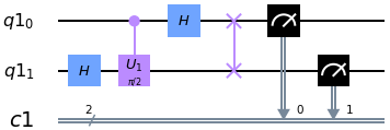
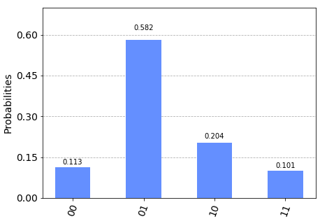
9 QFT . Fourier β₀ = 0.574,β₁ = 0.037,β₂ = 0.306,β₃ = 0.138 QFT 15.

Figure 16. QFT

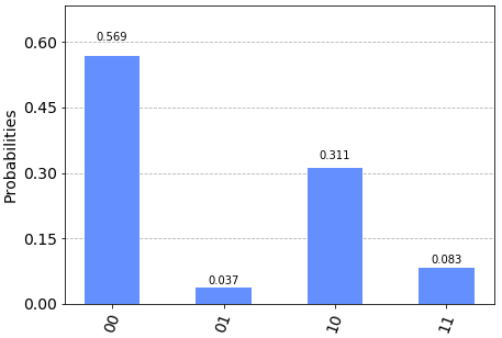
QFT β₀ = 0.569,β₁ = 0.037,β₂ = 0.311,β₃ = 0.083. QFT DFT.

5.6

. Hamiltonian Schrödinger ( [57, 58]. . ≈ 10²³ . . . QC .

Hamiltonian. Hamiltonian Bose-Einstein Schrödinger :

ℏ2- 2 ′ ℋBEC = − 2m ∇ + Vext(r)+ Uint(r− r ),

(37)

$-∂ ∂t$ \|Ψ_BEC⟩	= $1- iℏ$ $[$ − $-ℏ2 2m$ ∇² + V_ext(r) + U_int(r −r′) $]$ \|Ψ_BEC⟩	(38)
\|Ψ_BEC⟩	= e^{−iℋ_BECt∕ℏ}\|Ψ_BEC0⟩.	(39)

. QC ( #7) [3] . Trotter ( Lie-Trotter-Suzuki). P Q Hermitian ( ) t

lim (eiPt∕NeiQt∕N)N = ei(P+Q)t. N →∞

(40)

$ei(P+Q)δt = (eiPδteiQδt) +𝒪(δt2) iPδt∕2iQδt iPδt∕2 3 = (e e e )+ 𝒪(δt).$

(41)

ℋ_BEC ℋ_BEC = ∑_i=1ⁿℋ_i Hamiltonian Hilbert . [ℋ_i,ℋ_j] = 0∀i, j ℏ = 1

e−iℋBECt = e−iℋ1te−iℋ2t...e−iℋnt.

(42)

e−iℋBECt = e−iℋ1t∕2e−iℋ2te−iℋ1t∕2 + 𝒪(δt3).

(43)

. QC.

Landau . ODEs PDEs :

$∂u1 ---- ∂t$ + u₁ ⋅∇u₁	= −∇ $($ $p1 --- ρ1$ $)$ ,	(44)
$∂u2- ∂t$ + u₂ ⋅∇u₂	= −∇ $($ $-p2 ρ2$ $)$ + $-ν ρ2$ ∇²u₂.	(45)

1 2 . .

Madelung BEC . Gross-Pitaevskii

$∂ 1[ ℏ2 2 ∂t|Ψcond⟩ = iℏ − 2m-∇ + Vext(r)+ ] + Uint|⟨Ψcond|Ψcond⟩||Ψcond⟩.$

(46)

: (a) BEC T ∼ 0 Ψ_BEC ≈ Ψ_cond. (b) . (c) U_int = Uδ(r −r′). . [57, 58].

. l .

dl dt = usa + uf,

(47)

u_sa u_f . QC Biot-Savart

∮ ′ ui = Γ-- -(l−-l) × dl, 4π |l− l′|3

(48)

u_sa Γ .

Landau . f_mf f_T. . ( F = f_mf + f_T:

$∂u1- ∂t$ + u₁ ⋅∇u₁	= −∇ $($ $p1- ρ1$ $)$ −F,	(49)
$∂u2- ∂t$ + u₂ ⋅∇u₂	= −∇ $($ $p2- ρ2$ $)$ + $-ν ρ2$ ∇²u₂ + $ρ1 ρ2$ F.	(50)

. CFD Stokes Gauss-Seidel Jacobi. Ax = B HHL. . x 0. . QC .

A. (VQE). . . VQE . . [25, 40, 59].

P |ψ_p⟩. |ψ_p⟩ P|ψ_p⟩ = p|ψ_p⟩ p . P Hamiltonian Hermitian . Hamiltonian ⟨ψ|ℋ|ψ⟩ ≥ 0. p_min ≤ ⟨ψ|ℋ|ψ⟩ (≥ 0) 2.
QPU CPU .

B. (QAOA): . QAOA . x = x₁...x_n x_i ∈ {0,1} E(x) . E(x) : {0,1}ⁿ $↦→$ ℝ. QAOA [60, 40, 25] α

α =-E(x)≥ α . Emax opt

(51)

Figure 17.

: ℋ,|ψ(k)⟩,k(parameter),𝜖(tolerance)

: |ψ(k)⟩_opt,E_opt

return |ψ(k)⟩_opt,E_opt

CLASSICAL_OPTIMISER(|ψ(k)⟩):

|ψ(k)⟩ k CPU

return |ψ(k)⟩_opt

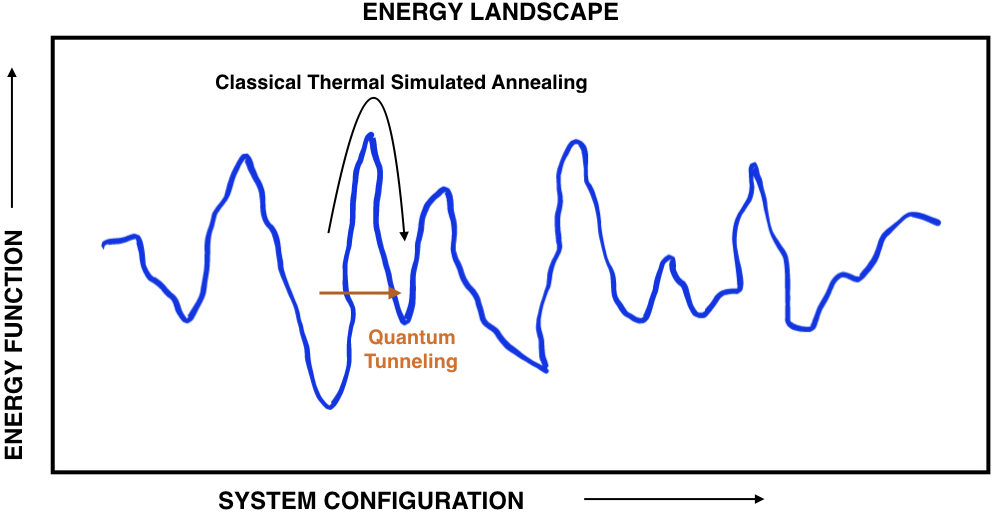
C. : ( ) DWave. . . Monte Carlo “” 16.

DWave . [61, 54] . Navier-Stokes [62]. NS Ax = B . (QUBO) DWave.

Figure 18.

DWave 5000 . .

Figure 19. QCs

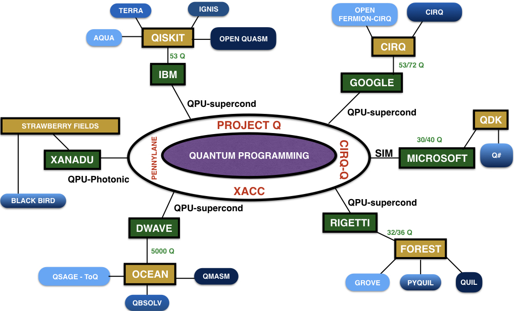
(a) (b) QCs . . QCs (QPU) . QPU .

QC. QC . . 17. . Qiskit IBMQ transmon. cbit. .

IBMQ 54 .

QFT: DNS FFT . 54 FFT 2⁵⁴ ≈ 10¹⁶ . DNS .
DNS: 54
1. 1D: ≤ 10¹⁶
2. 2D: ≤ 10⁸ ×10⁸
3. 3D: ≤ 10⁵ ×10⁵ ×10⁵
DNS .

DNS.

QCFD. . QCFD. QCs IBMQ . QC . QC . QCFD . QPU CPU GPU. .

IBM Q IBM Q Experience . IBM IBM Q. Jörg Schumacher Dhawal Buaria Kartik P Iyer .

References

[1] R.P. Feynman, Int. J. Theor. Phys. 21, 467 (1999). [2] J. Preskill , Quantum 2, 79 (2018). [3] M.A. Nielsen and I.L. Chuang, Quantum Computation and Quantum Information, 10th Anniversary Edition, (Cambridge University Press, 2002). [4] S.A. Orszag and G.S. Patterson, Jr, Phys. Rev. Lett. 28, 76 (1972). [5] R.S. Rogallo, National Aeronautics and Space Administration, 81315 (1981). [6] S.B. Pope, Turbulent Flows (Cambridge University Press, 2001). [7] P.K. Yeung, D.A. Donzis and K.R. Sreenivasan, Phys. Fluids, 17, 081703 (2005). [8] K.P. Iyer, J.D. Scheel, J. Schumacher and K.R. Sreenivasan, Proc. Natl. Acad. Sci. 117, 7594 (2020). [9] J. Smagorinsky, B. Galperin and S. Orszag, Evolution of Physical Oceanography (Cambridge University Press, 1993). [10] C. Meneveau and J. Katz, Annu. Rev. Fluid Mech. 32, 1 (2000). [11] P.A. Davidson, Turbulence: An Introduction for Scientists and Engineers, 2nd Edition (Oxford University Press, 2015). [12] S. Succi, R. Benzi and F. Higuera, Physica D 47, 219 (1991). [13] S. Succi, The Lattice Boltzmann Equation for Fluid Dynamics and Beyond (Oxford University Press, 2001). [14] D.A. Meyer, J. Stat. Phys. 85, 551 (1996). [15] D.A. Meyer, Phil. T. Roy. Soc. A 360, 395 (2002). [16] B.M. Boghosian and W. Taylor IV, Int. J. Mod. Phys. C 8, 705 (1997). [17] B.M. Boghosian and W. Taylor IV, Phys. Rev. E 57, 54 (1998). [18] B.M. Boghosian and W. Taylor IV, Physica D 120, 30 (1998). [19] S. Lloyd, Science 273, 1073 (1996). [20] D.S. Abrams and S. Lloyd, Phys. Rev. Lett. 79, 2586 (1997). [21] J. Yepez, Int. J. Mod. Phys. C 9, 1587 (1998). [22] J. Yepez, Phys. Rev. E 63, 046702 (2001). [23] J. Yepez, Int. J. Mod. Phys. C 12, 1285 (2001). [24] J. Yepez, J. Stat. Phys. 107, 203 (2002). [25] IBM, IBMQ Qiskit Textbook,
https:qiskit.org/textbook/preface.html [26] R. Benzi, S. Succi and M. Vergassola, Phys. Rep. 222, 145 (1992). [27] A Mezzacapo, M. Sanz, L. Lamata, I.L. Egusquiza, S. Succi and E. Solano, Sci. Rep. 5, 13153 (2015). [28] F. Fillion-Gourdeau, H.J. Herrmann, M. Mendoza, S. Palpacelli and S. Succi, Phys. Rev. Lett. 111, 160602 (2013). [29] S.L. Sondhi, S.M. Girvin, J.P. Carini and D. Shahar, Rev. Mod. Phys. 69, 315 (1997). [30] T.H. Hsieh, Student Review (2) 1, (2016). [31] O. Aharony, S.S. Gubser, J. Maldacena, H. Ooguri and Y. Oz, Phys. Rep. 323, 183 (2000). [32] A.M. Polyakov, Contemp. Concepts Phys. 3, 1 (1987). [33] R.D. Somma, C.D. Batista and G. Ortiz, Phys. Rev. Lett. 99, 030603 (2007). [34] M. Plesch and Č. Brukner, Phys. Rev. A 83, 032302 (2011). [35] V.V. Shende, S.S. Bullock and I.L. Markov, IEEE TCAD 25, 1000 (2006). [36] J.A. Cortese and T.M. Braje, arXiv preprint, arXiv:1803.01958, (2018). [37] K. Vogel and H. Risken, Phys. Rev. A 40, 2847 (1989). [38] U. Leonhardt, Measuring the quantum state of light 22, (Cambridge University Press, 1997). [39] W. Nawrocki, Quantum standards and instrumentation (Springer, Heidelberg, 2015). [40] P.J. Coles et al., arXiv preprint, arXiv:1804.03719, (2018). [41] G. Brassard, P. Hoyer, M. Mosca and A. Tapp, International Colloquium on Automata, Languages, and Programming 820, (Springer, 1998). [42] L.K. Grover, Phys. Rev. Lett. 79, 325 (1997). [43] G. Brassard, P. Hoyer, M. Mosca and A. Tapp, Contemp. Math. 305, 53 (2002). [44] H. Buhrman and R. palek, Proc. 17th Annual ACM-SIAM Symp. on Discrete Algorithm (Society for Industrial and Applied Mathematics, 2006). [45] S.P. Jordan, Phys. Rev. Lett. 95, 050501 (2005). [46] S. Jordan, Quantum Algorithm Zoo,
https://quantumalgorithmzoo.org/. [47] A.W. Harrow, A. Hassidim and S.Lloyd, Phys. Rev. Lett. 103, 150502 (2009). [48] D.W. Berry, J. Phys. A-Math. Theor. 47, 105301 (2014). [49] P.C.S. Costa, S. Jordan and A. Ostrander, Phys. Rev. A 99, 012323 (2019). [50] Y. Cao, A. Papageorgiou, I. Petras, J. Traub and S. Kais,New J. Phys. 15, 013021 (2013). [51] J.M. Arrazola, T. Kalajdzievski, C. Weedbrook and S. Lloyd, Phys. Rev. A 100, 032306 (2019). [52] L. Ruiz-Perez and J.C. Garcia-Escartin, Quantum Inf. Process. 16, 152 (2017). [53] S. Hadfield, arXiv preprint, arXiv:1805.03265, (2018). [54] DWave,
https://docs.dwavesys.com/docs/latest/c_gs_2.htmll. [55] A. Montanaro, NPJ Quantum Inf. 2, 1 (2016). [56] G. Xu, A.J. Daley, P. Givi and R.D. Somma, AIAA J. 56 687, (2018). [57] C.F. Barenghi, L. Skrbek and K.R. Sreenivasan, Proc. Natl. Acad. Sci. 111, 4647 (2014). [58] C.F. Barenghi, V.S. Lvov and P. E. Roche, Proc. Natl. Acad. Sci. 111, 4683 (2014). [59] A. Peruzzo, et al., Nat. Commun. 5, 4213 (2014). [60] E. Farhi, J. Goldstone and S. Gutmann, arXiv preprint, arXiv:1411.4028, (2014). [61] D.A. Battaglia, G.E. Santoro and E. Tosatti, Phys. Rev. E 71, 066707 (2005). [62] N. Ray, T. Banerjee, B. Nadiga and S. Karra, arXiv preprint, arXiv:1904.09033, (2019).