Saif Eddin Jabari*^1,2, Nikolaos M. Freris³, and Deepthi Mary Dilip⁴

¹New York University Abu Dhabi, Saadiyat Island, P.O. Box 129188, Abu Dhabi, U.A.E.
²New York University Tandon School of Engineering, Brooklyn NY
³School of Computer Science and Technology, University of Science and Technology of China, Diansan Building, West Campus, 443 Huangshan Road, Hefei, Anhui, 230027 China
⁴BITS Pilani, Dubai Campus, Dubai International Academic City, Dubai, U.A.E.

*Corresponding author, E-mail: sej7@nyu.edu

Abstract

. . . . . . Mittag-Leffler . ( ) . .

: Mittag-Leffler .

1

. . . ([Du et al., 2012, Ramezani and Geroliminis, 2012, 2015]).

: Kharoufeh and Gautam [2004] . Carey and Ge [2005a] LWR [Carey and Ge, 2005b]. Ghiani and Guerriero [2014] Ichoua Gendreau Potvin (IGP) [Ichoua et al., 2003] . Gómez et al. [2016] (VRPSTT). Zheng et al. [2017] .

. ( ) ( ) ( ). () .

( ) [Richardson and Taylor, 1978, Rakha et al., 2006, Pu, 2011, Arezoumandi, 2011] [Polus, 1979, Kim and Mahmassani, 2014, 2015] Weibull [Al-Deek and Emam, 2006]. . [Hofleitner et al., 2012a, Kazagli and Koutsopoulos, 2013, Ji and Zhang, 2013, Feng et al., 2014]. [Rakha et al., 2011, Hofleitner et al., 2012b, Hunter et al., 2013, Yang et al., 2014]. [Guo et al., 2010, Wan et al., 2014, Rahmani et al., 2015]. (EM) [Redner and Walker, 1984] . (MCMC) [Chen et al., 2014] . EM . .

( ) [Emam and Al-Deek, 2006, Fosgerau and Fukuda, 2012, Jenelius and Koutsopoulos, 2013, Xu et al., 2014, Kim and Mahmassani, 2015, Jenelius and Koutsopoulos, 2015, Taylor, 2017]. . . . .

. . [Mukherjee and Vapnik, 1999] [Lin et al., 2013] [Chen et al., 2004, 2008]. ( ) [Hofleitner et al., 2013, 2014].

. [Dilip et al., 2017]. . . ( ) . . ( ).

( ) . -. . ℓ₁− [Tibshirani, 1996] . (i) (ii) .

: 2. 3 . ( ) Mittag-Leffler 4. 5 6 . 7 () ( ) 8 . .

: A B C D E .

2

2.1

x₁ x₂ . C(x) x. C(x₂) − C(x₁). C . P(x)

∫ x2 C(x2)− C (x1) = P (x)dx, x1

(1)

dC-(x) P (x) = dx .

(2)

P(x) x ( ). x x: r V(r) Q(r) = rV(r) . P :

P(r) = --r-- = --1--. Q(r) V (r)

(3)

r→ 0 P(r) → v_fr⁻¹ v_fr .
r→r_jam P(r) →r_jam .
P(r) r∈(0, r_jam).
P(r) r.

(i) - (iii) [Del Castillo and Benitez, 1995]. (iv)

dP(r)- d----r-- --1-- -1---dQ-(r) dr = dr(Q (r)) = Q (r)(1− V(r) dr ),

(4)

0 ≤r≤r_jam V(r) ≥ dQ(r)/dr. Q(⋅)

dP(r)-≥ 0 dr

(5)

0 ≤r≤r_jam P(⋅) . Newell-Franklin [Newell, 1961, Franklin, 1961] 1.

V(r) = v_fr $($ 1 − e^{( −1)} $)$ ,

(6)

v_b .

1: - v_fr = 100 / v_b = −20 / r_jam = 150 /.

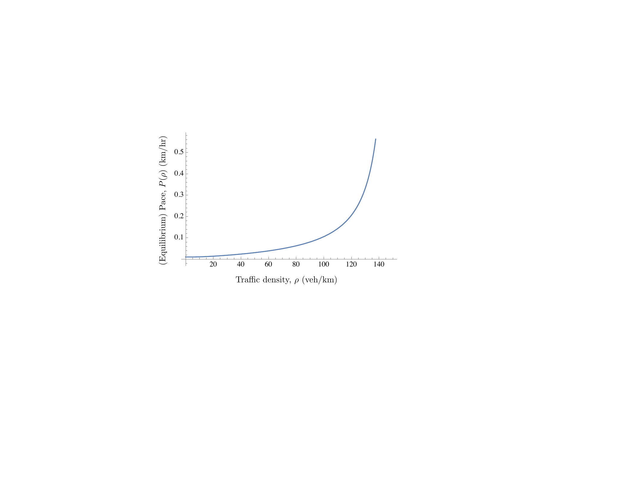
[v_fr⁻¹, ). [Polus, 1979, Kim and Mahmassani, 2014, 2015] [Richardson and Taylor, 1978, Rakha et al., 2006, Pu, 2011, Arezoumandi, 2011] . .

2.2

[Carey and Ge, 2005b] Lighthill and Whitham [1955] Richards [1956] ( LWR) . P(x) ≡ P $($ r(x), x $)$ . (1)

∫ x2 C (x2)− C (x1) = P (r (x),x )dx. x1

(7)

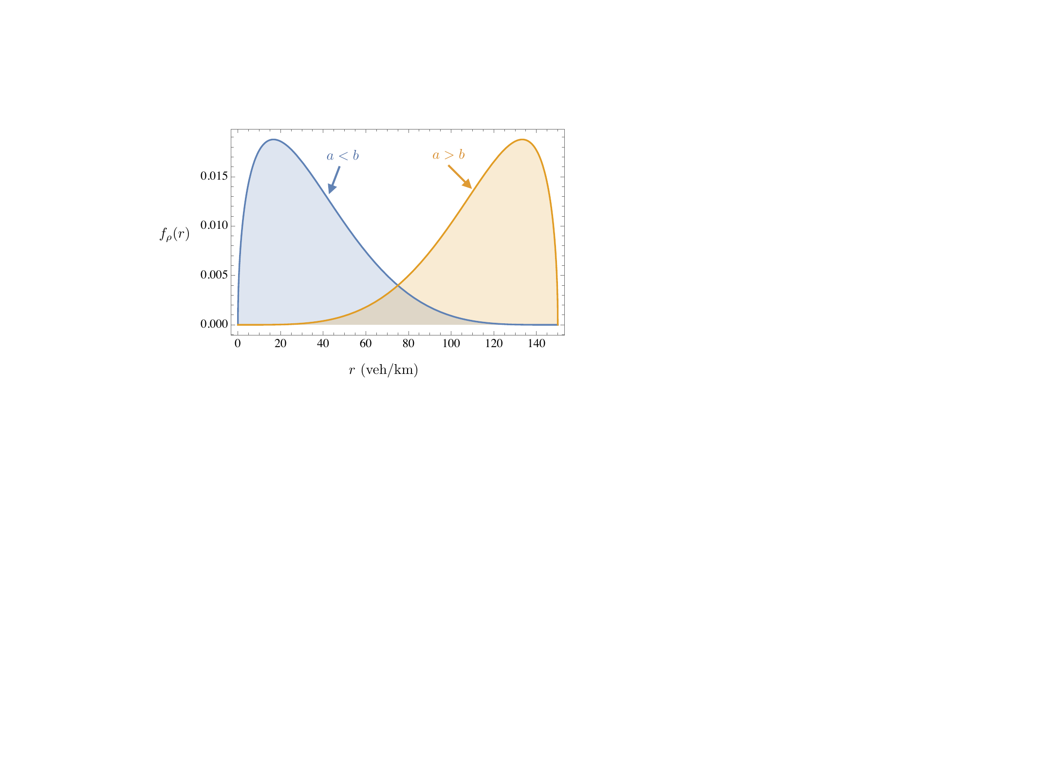
() . r(x) x P(r(x) ≤ 0) = P(r(x) ≥r_jam) = 0 . . Haight [1963] . . a = b = 1 . a < b a > b . (PDF) a, b r_jam :

1 fr(r) = 1{r∈[0,rjam]}-a+b−1------ra−1(rjam − r)b− 1, rjam B(a,b)

(8)

B 2.

2: f _r a < b ( ) a > b ( ). r_jam = 150 /.

Newell-Franklin (6) P PDF f _r . PDF f _P

f _P (t) = 1_{{tv_fr≥1}} f _r $($ P⁻¹(t) $)$ $dP-−1(t) dt$ .

(9)

P⁻¹ ( ). x P(x) P .

2.3

P ( Weierstrass). {z_k}_k≥0 e₁, e₂ > 0

$|| |$ P(r) − _k=0z_kr^k $|| |$ ≤e₁

(10)

r∈[0, r_jam −e₂]. r_jam P ( P r_jam).

k P (r) ≈ zkr k=0

(11)

r∈[0, r_jam). P(x) j_P (s) ≡Ee^isP(r) x i ≡ $--- √ − 1$ . e^isP(r) Maclaurin

j_P (s)

= E _j=0 $j (is)- j!$ $($ P(r) $)$ ^j = 1 + E _j=1 $j (is)- j!$ $($ P(r) $)$ ^j.

(12)

(11)

$($ P(r) $)$ ^j

= $($ _k=0z_kr^k $)$ ^j = _k₁=0… _{k_j=0} _l=1^jz_{k_l}r^k₁+…+k_j = _m
=0 $($ _{k₁+…+k_j=m} $( m ) k ... k 1 j$ _l=1^jz_{k_l} $)$ r^m.

(13)

{z_k}_k≥0 ( ) m _l=1^jz_{k_l} C_m. _{k₁+…+k_j=m} $( m ) k1 ... kj$ = j^m.

j_P (s) = 1 + E _j=1 $j (is) j!$ _m=0C_mj^mr^m = 1 + _m=0 _j=1 $j (is)- j!$ C_mj^mEr^m.

(14)

PDF (2) m :

Erm = rm B(a-+-m,b)-= rm G(a-+-b)G(a+-m-), jam B(a,b) jam G(a)G(a + b+ m )

(15)

G . b_m ≡ a + b + m

j_P (s) = 1 + _m=0C_mr_jam^m $G(a+-b)G-(a-+-m-) G(a)$ _j=1 $j (is)- j!$ $m ----j---- G (bm + j)$ $G(bm-+-j) G (bm)$ .

(16)

$～C$ _m m ( j)

_j=1 $j (is)- j!$ $m ----j---- G(bm + j)$ $G-(bm +-j) G(bm )$ = $C～$ _m _j=1 $j (is) j!$ $G(bm-+-j) G (bm)$ .

(17)

q_m ≡ C_mr_jam^m $G(a+b)G(a+m-)～Cm- G(a)$

j_P (s) = 1 + _m=0q_m _j=1 $j (is) j!$ $G(bm-+-j) G(bm )$ .

(18)

(1) bsj_G (s)

− b (is)j jG(b-+-j)- jG (s) = (1 − sis) = j! s G (b) j=0

(19)

(2) .

f _X(x) = _m=0q_m f _m(x)

(20)

X ℛ⊆R { f _m}_m≥0

j_X(s)

= ∫ _ℛe^isx f _X(x)dx = ∫ _ℛe^isx _m=0q_m f _m(x)dx = _m=0q_m ∫ _ℛe^isx f _m(x)dx = _m=0q_mj_m(s),

(21)

{j_m}_m≥0 . f _P s= 1 {b_m}_m≥0 _m=0q_m = 1.

j_P (s) = _m=0q_m _j=0 $j (is)- j!$ $G-(bm-+--j) G(bm )$ = _m=0q_m(1 − is)^−b_m.

(22)

PDF bs

1 t t fG(t;b,s ) = 1{t≥0}-----(-)b−1e− s. sG(b ) s

(23)

f _P (t) = _m=0q_m f _G (t; b_m, 1).

(24)

: P x / - [Jabari et al., 2014, 2018, Zheng et al., 2018]. x₁ ≤x ≤ x₂

-- -- ∫ x2 P (r (x ),x)(x2 − x1) = x P(r(x),x)dx. 1

(25)

x₁ x₂ "" "." C(x₂) − C(x₁) = P $($ r(x), x $)$ (x₂ − x₁) .

C(x₂) − C(x₁) = P $($ r(x), x $)$ (x₂ − x₁) = _k=0 $～z$ _kr^k,

(26)

{ $～z$ _k}_k≥0 .

f _T(t) = _m=0q_m f _G (t; b_m, 1),

(27)

f _T . (27).

( Gaussian biweight Epanechnikov) . .
{b_m}_m≥0 P {q_m}_m≥0. .
s= 1 m . {b_m − 1}_m≥0.
:
1. : m b_m. . 4.1.
2. ( ) s= 1. 4.3 .
3. . M < M . 1 2 B _m=0^Mq_m = 1.

3

. . . .

3.1 :

S T₁, …, T_S () f . (PW) [Parzen, 1962, Cacoullos, 1966, Raudys, 1991, Silverman, 1986] t :

S ^f(t) = 1- k (t− T), S j=1 h j

(28)

k_h ( ) h h . "" . k_h ≡dd Dirac delta $1S$ _j=1^Sd(t − T_j) h = 0. k_h h² . h ( [Lacour et al., 2016] ).

Parzen (PW) . PW . . PW ( ) ( ) ( ).

3.2

-- M− 1 f(t) = qmfm (t), m=0

(29)

{f_m}_m=0^M−1 (M ) {q_m}_m=0^M−1 . M (29) . f ( ) q= [q₀…q_M−1]^⊤ PW h. :

M− 1 minimize 1∥^f − qmfm∥2 + w ∥q∥1, q∈W 2 m=0 2

(30)

W⊆R^M M w ≥ 0 . L₂− ( ) ℓ₁− ( ) .

1 M−1 1 ∫ M −1 --∥^f − qmfm ∥22 = -- (^f(t)− qmfm (t))2dt. 2 m=0 2 R+ m=0

(31)

∥ $^ f$ − _m=0^M−1q_mf_m∥₂² : L₂− () () $^ f$ f . ℓ₁− : ∥⋅∥₁ q [Tibshirani, 1996] . wq (30).

3.3

(30) . ( ) ( t_n n ). : t[0, T_max] {t_n}_n=0^N−1 t t $↦→$ t_n. t t t_n . PDFs $^f$ f N $^p$ p. t ≥ 0

M− 1 f(t) ≈ p- = qmfm (t (t)). t(t) m=0

(32)

M {t_m}_m=0^M−1 . {t_m}_m=0^M−1 M ( ) M > N. {t_m}_m=0^M−1 ∪_m=0^M−1{t_m}⊆{t_n}_n=0^N−1 {t_m}_m=0^M−1 M′ M′≤ N. ( 4) M = M′≤ N.

M : f_n,m ≡ c_n,mf_m(t_n) c_n,m m . PW $^p$ _n = a_n $^f$ (t_n). a_n n a_n ≡DD ( a_n ≡ 1). ( {c_n,m}) 4.2 4.3. F≡[f_n,m] ∈R₊^N×M,

-- p = Fq

(33)

():

N−1 M− 1 M −1 minimize 1∥^p − Fq ∥2+ w ∥q∥ = 1- (^p − f q )2 + w |q |, q∈W 2 2 1 2 n=0 n m=0 n,m m m=0 m

(34)

() (LASSO) [Tibshirani, 1996].

4 Mittag-Leffler

3.2 2 2.3.

4.1

( ) ( ). [Chen, 2000] . : t (i) (b− 1)s t (ii) (iii) . . . : () t (b− 1)s= t b= 1 + $t s$ s > 0 m :

t- fm (t) = fG(tm;1+ s,s).

(35)

( ) :

-- M −1 t- M −1 ----1-----tm- ts − tms f(t) = qm fG(tm;1 + s,s) = qm sG(1 + t)( s ) e . m=0 m=0 s

(36)

4.2

. ∫ ₀ f _G (t_m; 1 + s⁻¹t, s)dt≠1: . p (PMF). $^p$ .

p . : $^p$ ∥ $p^$ −p∥₂² p _n=0^N−1p_n . (). .

(). _n=0^N−1p_n ≈ 1 . {f_n,m}_n=0^N−1 _n=0^N−1f_n,m ≈ 1 m ∈{0, …, M − 1} ( F ). {c_n}_n=0^N−1 .

1( ). D > 0 t_n ≡ nD t_m ≡ mD n ∈{0, 1, …}{m = 0, …, M − 1}. $～D$ ≡ $D s-$ f_n,m ≡ c_n f _G $($ t_m; 1 + n $D～$ , s $)$ c_n ≡s n. N < 0 < # < 1

N− 1 1− # ≤ f ≤ 1. n=0 n,m

(37)

Proof. $～D$ = 1 s≡D

N−1 N−1 N −1 1 tm ～ tm- fn,m = cnfG(tm;1 + n～D,s ) = ----------(--)nDe− s n=0 n=0 n=0G (1 + n～D ) s

(38)

1 ( ) N → (38) $tm s$ . N : X

tm- (M-−-1)D- {mtax}M−1 s = s = M − 1 m m=0

(39)

N (1 −#) X.

N ≡ min {n : P(X ≥ n) ≤ #}.

(40)

. □

(1) max _{m=0,…,M−1} $tm s$ N t_m t_m (2) N > M (3) _n=0^N−1f_n,m = 1 j ∈{0, …, M − 1} ( ) f_0,m ( m)

f0,m ≡ (#m + 1)e− tms ,

(41)

1 t #m = --(-m-)n. n=N n! s

(42)

#_m m #_M−1.

4.3 -

s. Mittag-Leffler. $～ D$ = 1 s . . e⁻ (23) Mittag-Leffler () [Haubold et al., 2011]:

tn En(t) ≡ ---------. n=0G(1 + nn)

(43)

Mittag-Leffler n= 1 E₁(t) ≡ e^t. (23) :

---1-- t- b− 1 -t n − 1 fM− L(t;b,s,n) = sG (b)(s ) [En((s ) )] ,

(44)

bsn . 2 1 ( ). {c_n,m}_n,m=0^,M−1 .

2( -). D {t_n}_n=01. {t_m, s_m}_m=0^M−1 c_n,m ≡s_m n, m. $～D$ _m ≡ $Dsm$

f_n,m ≡ c_n,m f _M−L(t_m; 1 + n $～D$ _m, s_m, $D～$ _m) = $1 -------～--- G(1 + nDm )$ $($ $tm --- sm$ $)$ ^{n _m} $[$ E_{_m} $($ $($ $tm --- sm$ $)$ ^_m $)$ $]$ ⁻¹

(45)

n = 0, … m = 0, …, M − 1. N < 0 < # < 1

N− 1 1− # ≤ fn,m ≤ 1. n=0

(46)

Proof. 0 ≤ m ≤ M − 1 $～X$ _m Hyper-Poisson [Chakraborty and Ong, 2017] p_{_m} a_m b_m:

1 P(～Xm = n) ≡ p～Xm(n;am,bm ) = anm------------------. G(1 + nbm)Ebm(am )

(47)

a_m ≡ $($ t_m/s_m $)$ ^_m b_m ≡ $～ D$ _m = D/s_m. m {f_n,m}_n=0 (45) .

N −1 lim fn,m = 1. N↑ n=0

(48)

N ≡ min ${$ n : P( $～X$ _m ≥ n) ≤#, for 0 ≤ m ≤ M − 1 $}$ = min ${$ n : P( $～X$ _M−1 ≥ n) ≤# $}$

(49)

. □

_n=0^N−1f_n,m = 1

～D − 1 f0,m ≡ (～#m + 1)[E～Dm((tm/sm ) m)] ,

(50)

-----1----- -tm- n～Dm ～#m = G (1+ nD～ )(sm ) . n=N m

(51)

Mittag-Leffler (ML) ( s_m) t_m ( ) M > N . {s_m}_m=0^M−1 . N > M′ M′ {t_m}_m=0^M−1.

5

LASSO () (34) W= R₊^M ( ) W= {q∈R₊^M| _m=0^M−1q_m = 1} ( ). . ( ). W= {q∈R₊^M| _m=0^M−1q_m = 1} :

1 2 ⊤ miniqm≥i0ze 2∥^p − Fq∥ 2 + w1 q ⊤ subject to 1 q = 1,

minimize 1∥^p− Fq ∥2 q≥0 2 2 subject to 1⊤q = 1

(1 1 s M). w. W= R₊^M . _n=0^N−1p_n = 1 () . B.

LASSO (34) [Boyd and Vandenberghe, 2004] . CVX [Grant and Boyd, 2014] : Nesterov [2013] [Beck and Teboulle, 2009, Wright et al., 2009] (ADMM) [Parikh and Boyd, 2014] [Afonso et al., 2010] [Kim et al., 2007]. [Sopasakis et al., 2016].

W= R₊^M LASSO ( ):

1 2 ⊤ minimMi+z1e 2∥^p − Fq ∥2 + w1 q, q∈R+

(52)

. C. (l1_ls) [Kim et al., 2007]. − _m=0^M log(q_m)

z M M minimize -∥^p − Fq ∥22 + zw qm − log(qi), q∈RM+1 2 m=0 m=0

(53)

z →+.

w D E .

6

. . ( ) . [Freris et al., 2013a,b] [Sopasakis et al., 2016] LASSO .

M ( q) S ( ML). (i) Parzen (ii) LASSO (52). . (52) $^ q$ LASSO ( Parzen $^p$ ). 7.5. : (1) "" $^ q$ (2) ( ) . . . .

6.1

{T₁, T₂, …} {t_n}_n=0^N−1. K + 1 K K ∈Z₊. K LASSO

1 ^q(K) ∈ argmin -∥^p(K) − Fq ∥22 + w1⊤q. q∈W 2

(54)

F K ( ). $^q$ ^(K+1) $^q$ ^(K) . Parzen (28) :

^(K+1) --K---^(K ) --1--- f (t) = K + 1 f (t)+ K+ 1kh(t− TK+1).

(55)

k_h(t − t_j) t ∈{t_n}_n=0^N−1 j = 0, 1, …, N − 1. Y∈R^N×N ( j YY_j :

Yj = [kh(t0 − tj) ... kh(tN−1 − tj)]⊤.

(56)

$^p$ ^(K+1) $^p$ ^(K) T_K+1 O(N) :

(K+1) --K--- (K) --1--- ^p = K+ 1^p + K + 1 YTK+1,

(57)

Y_{T_K+1} ∈R^N Y () T_K+1.

6.2

. . ( ).

T_W^(j) j W. W {T₁, T₂, …} T_W^(j) ≡{T_j, …, T_j+W−1} T_W^(j+1) ≡{T_j+1, …, T_j+W} .

T_W^(j) $^p$ ^(j) j

^q(j) ∈ argmin 1∥^p(j) − Fq ∥2+ w1 ⊤q. q∈W 2 2

(58)

{ $^q$ ^(j)} : j LASSO j + 1. Parzen (28) t ∈R₊ j

j+W −1 ^f(j)(t) = -1- k (t − t). W l=j h l

(59)

PW k_h(t − T_j+W) k_h(t − T_j)

1 ^f(j+1)(t) = ^f(j)(t)+ ---[kh(t− Tj+W )− kh(t− Tj)]. W

(60)

$^p$ ^(j+1) $^p$ ^(j) O(N) :

(j+1) (j) 1-- ^p = ^p (t) + W (YTj+W − YTj),

(61)

Y_{T_j+W}, Y_{T_j} ∈R^N Y () T_j+W, T_j . (j + 1) . LASSO 7.5.

7

7.1

. ML. S ( ) S_test (RMSE_oos)

┌│ ----S--(------------)-- RMSE = │∘ -1-- test ^f(t)− -f(t ) 2. oos Stest j=1 j j

(62)

() : (0.5):

f(t) = 0.5 √-1---e− (t−26000)2-+ 0.5 0.2-e− 0.2|t−30|. 200p 2

(63)

S = 2000 S_test = 10, 000. [1, 300]s M′= 300. s_m {1, 2, …, 10} ( M = 10M′= 3000) Gaussian ML. N = 2M′= 600 [1, 600] . Matlab CVX [Grant and Boyd, 2014] . . ( Gaussian ML) PW ( Gaussian h = 1.5) 4.

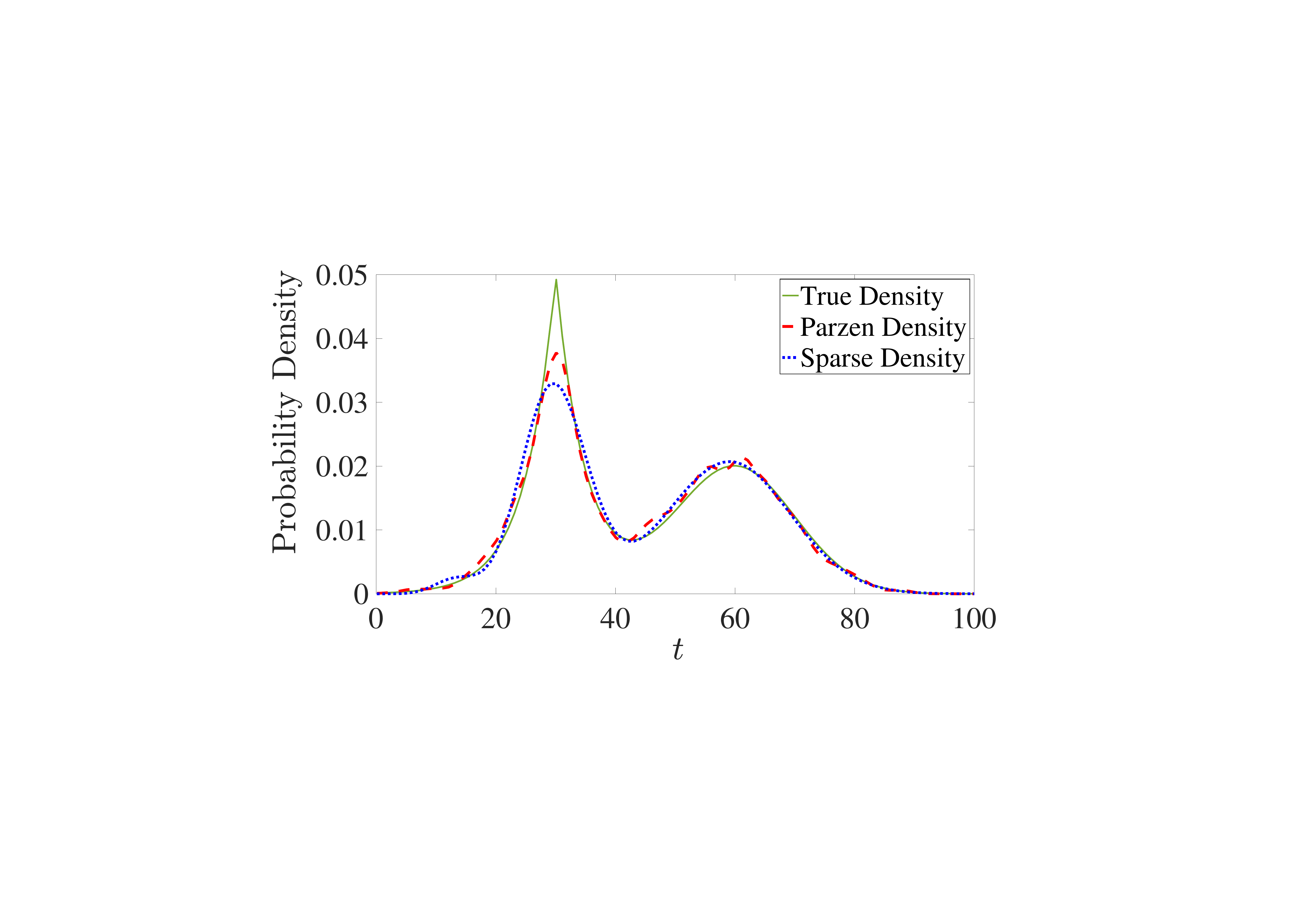
1 ( RMSE_oos ±1). 5 % 0.4 % Gaussian ML . ML 1. ML PW .

Table 1: .


Method	RMSE_oos	Number of mixture components


PW estimator	5.50e-04 ± 9.96e-05	2000
Sparse Gaussian estimator	3.3e-03 ± 1.92e-05	95
Sparse M-L Estimator	4.49e-04 ± 1.16e-04	7

7.2

7.2.1

(NGSIM) Peachtree Street (http://ngsim-community.org). 640 ( 2100) . . 4 . Peachtree 15: 12: 45 PM 1: 00 PM ( ) 4: 00 PM 4: 15 PM ( PM). . ( ).

NGSIM I-80 2005. 500 (HOV) ( Punzo et al. [2011] ). 30 5648 15: 4.00 PM 4.15 PM 5.00 PM 5: 15 PM 5: 15 PM 5.30 PM. .

7.2.2

. $^p$ ( PW) h () Silverman [1986]: h = 1.06VS^−1/5 ( V S ). ML M′= 300 s_m ∈{1, 2, 3, 4, 5} ( M = 1500 ).

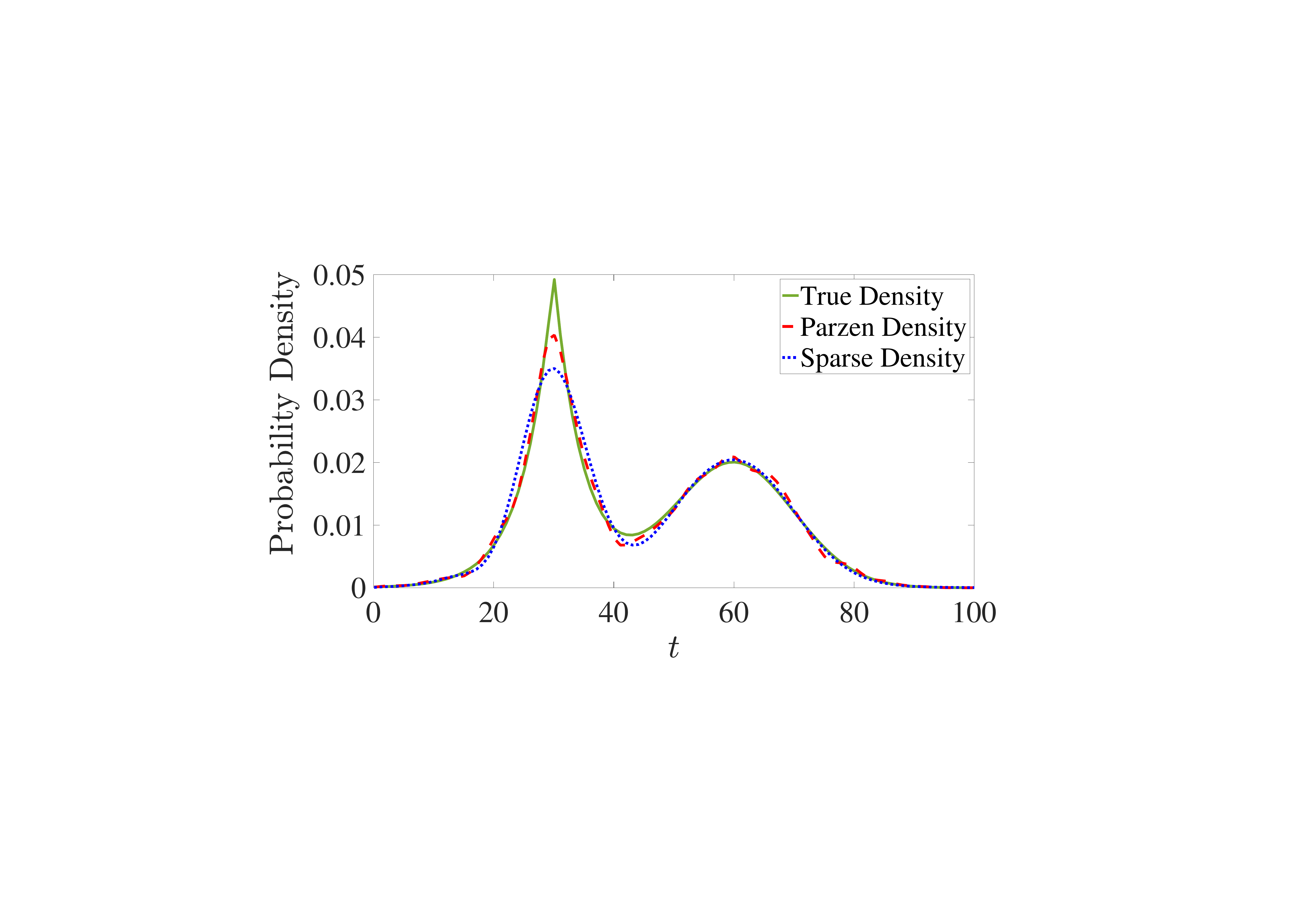
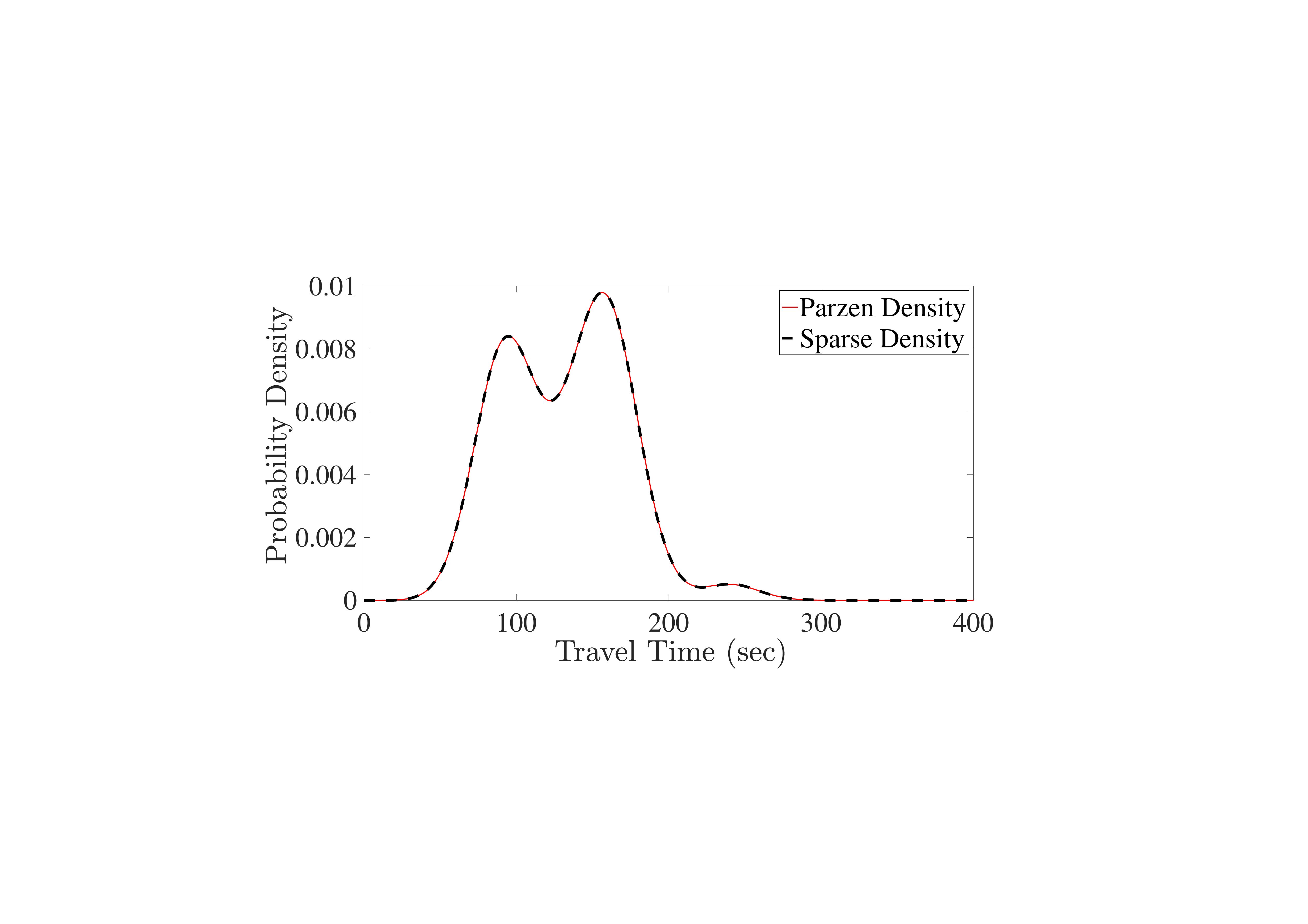
5 () PW ( ML) . PDF PW. : . PW (58 ) : ML 15: 1.

(EM) [Bishop, 2006] [Wan et al., 2014]. EM ( ) [Wu, 1983, Archambeau et al., 2003] [Biernacki et al., 2003]. EM ([Wan et al., 2014]). [Karlis and Xekalaki, 2003, Abbi et al., 2008]. ( 10⁻³) (RMSE)

┌│ -------------------- │ 1 N ( -- )2 RMSE = ∘ N- ^p(tj)− p(tj) . j=1

(64)

EM . . EM q. EM RMSE. 5 2 .

5: ( ) ( ) () ML Parzen () Parzen () Parzen () Parzen.

Table 2: : ML EM.


Method	No. mixture components	RMSE	Log-likelihood


Sparse M-L Estimator	4	0.0004	N/A
EM	2	0.0009	0.0021
EM	4	0.0012	0.0029
EM	6	0.0063	0.0152

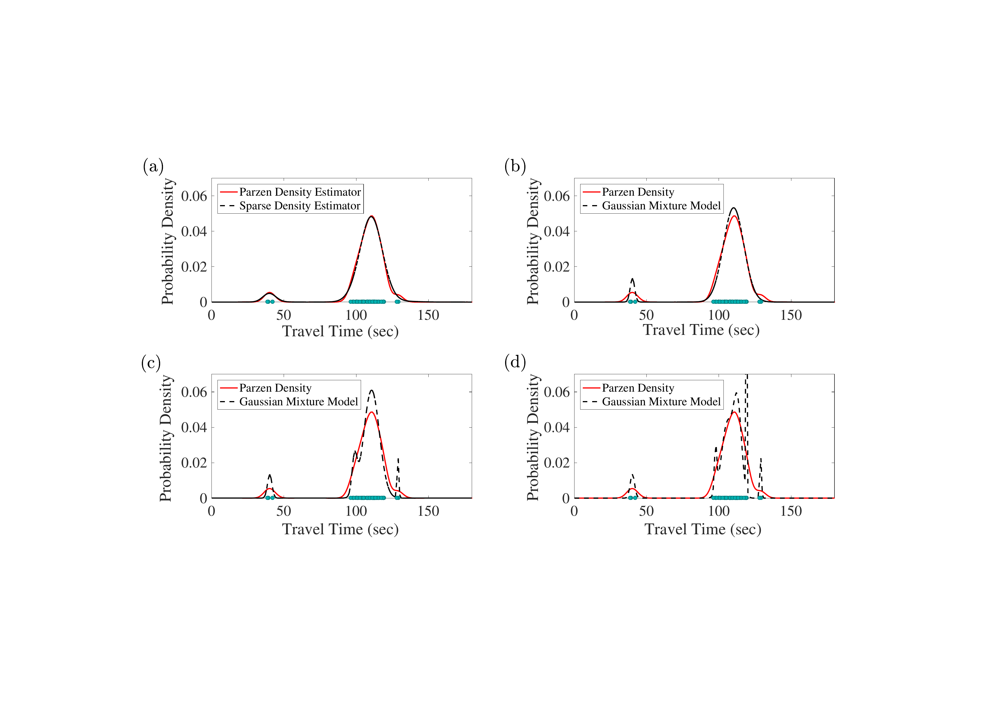
M-L EM . EM ( ) RMSE . EM . EM. ( .) . 6 ( I-80): RMSE EM ( ML w ).

7.3

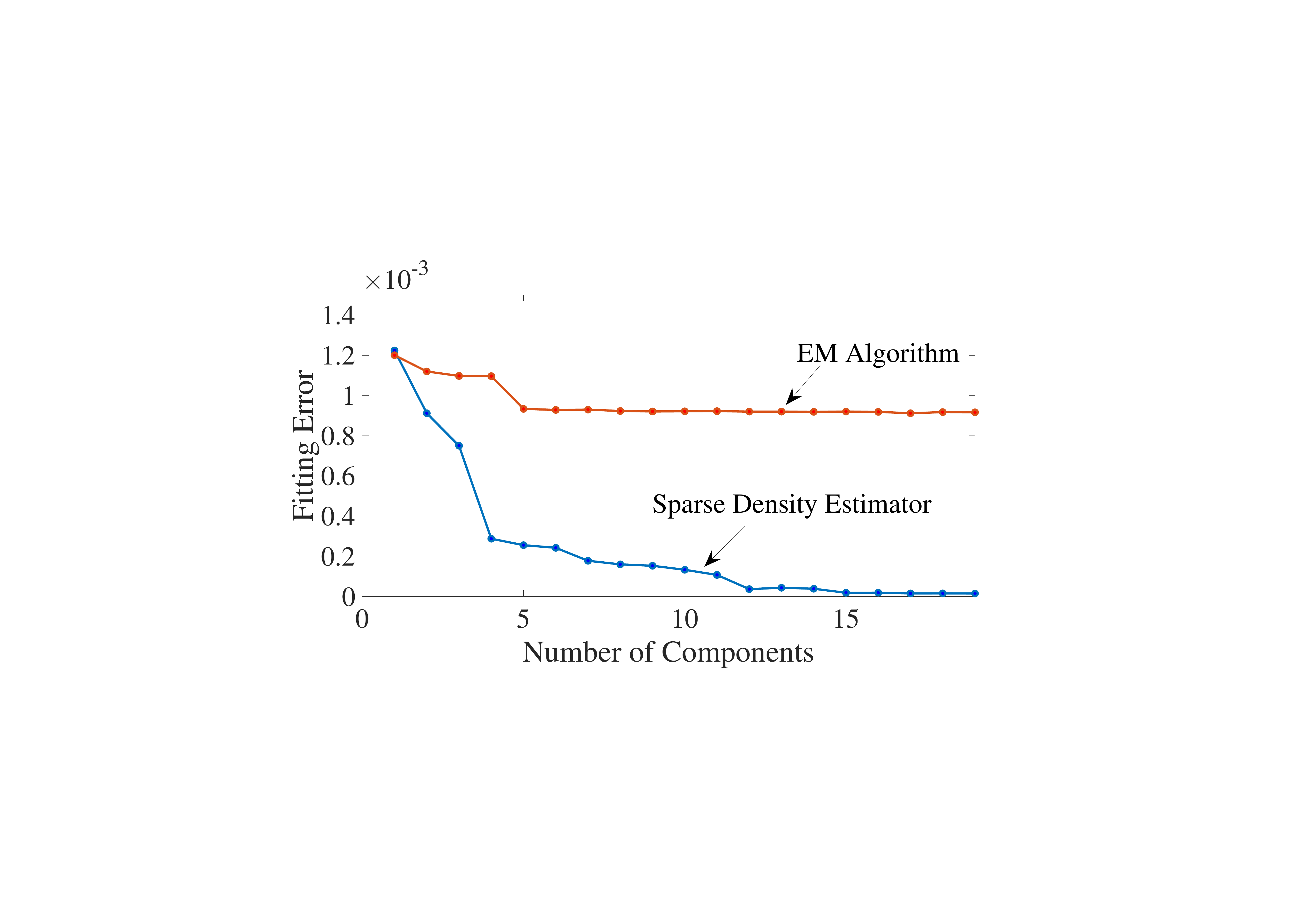
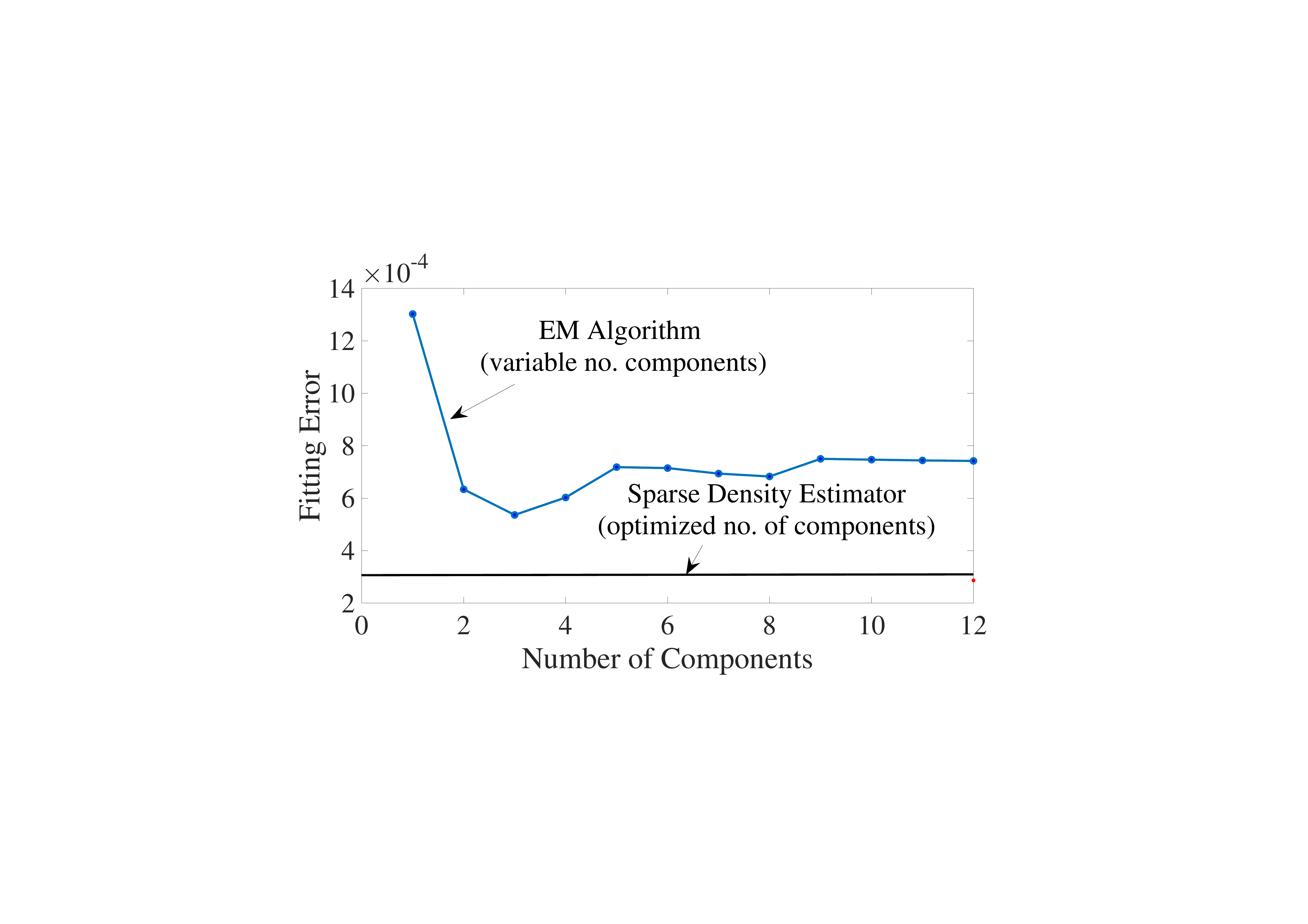
I-80: I-80 ( ): (i) (ii) ( 4 : 1 ). ( ) . . 7: 7 () PW ML ( 12 ) 7 () (RMSE) EM 1-12. EM .

ℓ₂− Peachtree ( ). M = 1500 M-L (M′= 300 s_m ∈{0.2, 0.3, 0.5, 1, 1.5}). ℓ₂ $w～$ {5 ⋅ 10⁻⁵, 5 ⋅ 10⁻⁴, 5 ⋅ 10⁻³, 5 ⋅ 10⁻², 5 ⋅ 10⁻¹} 5 : 1.

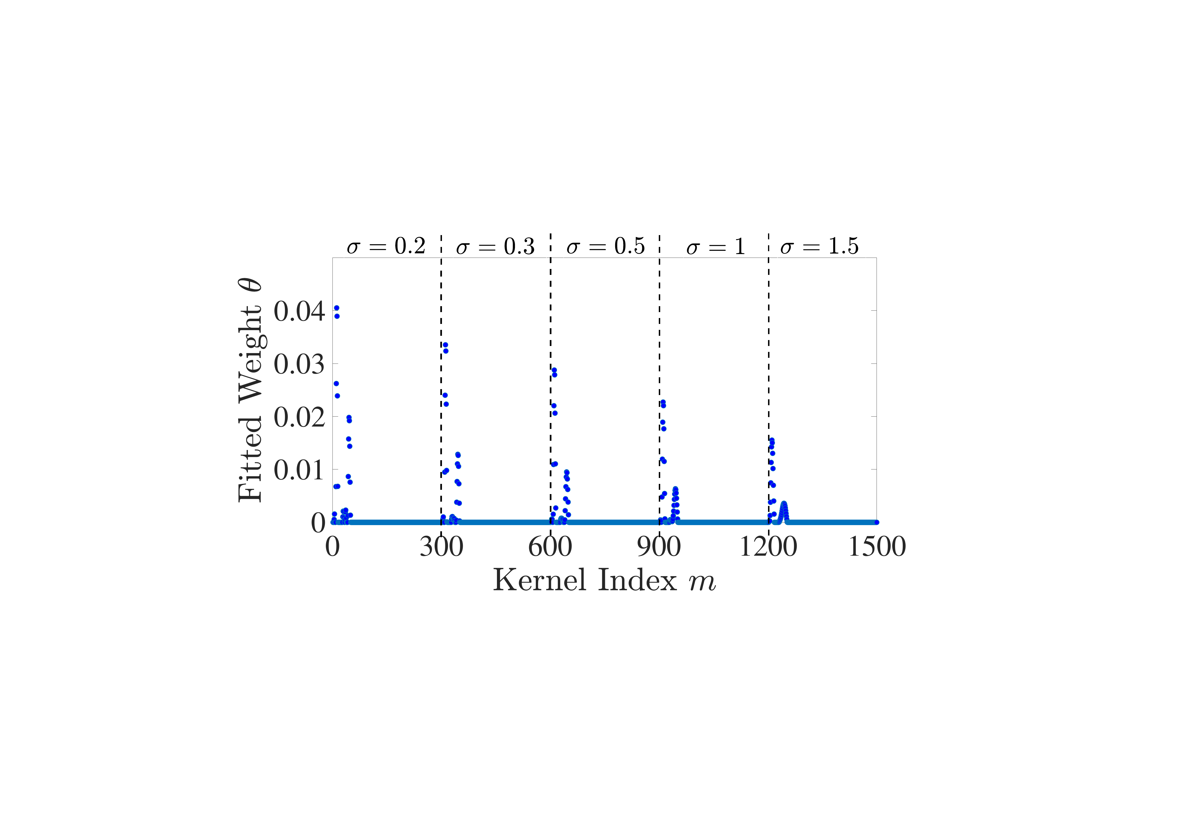
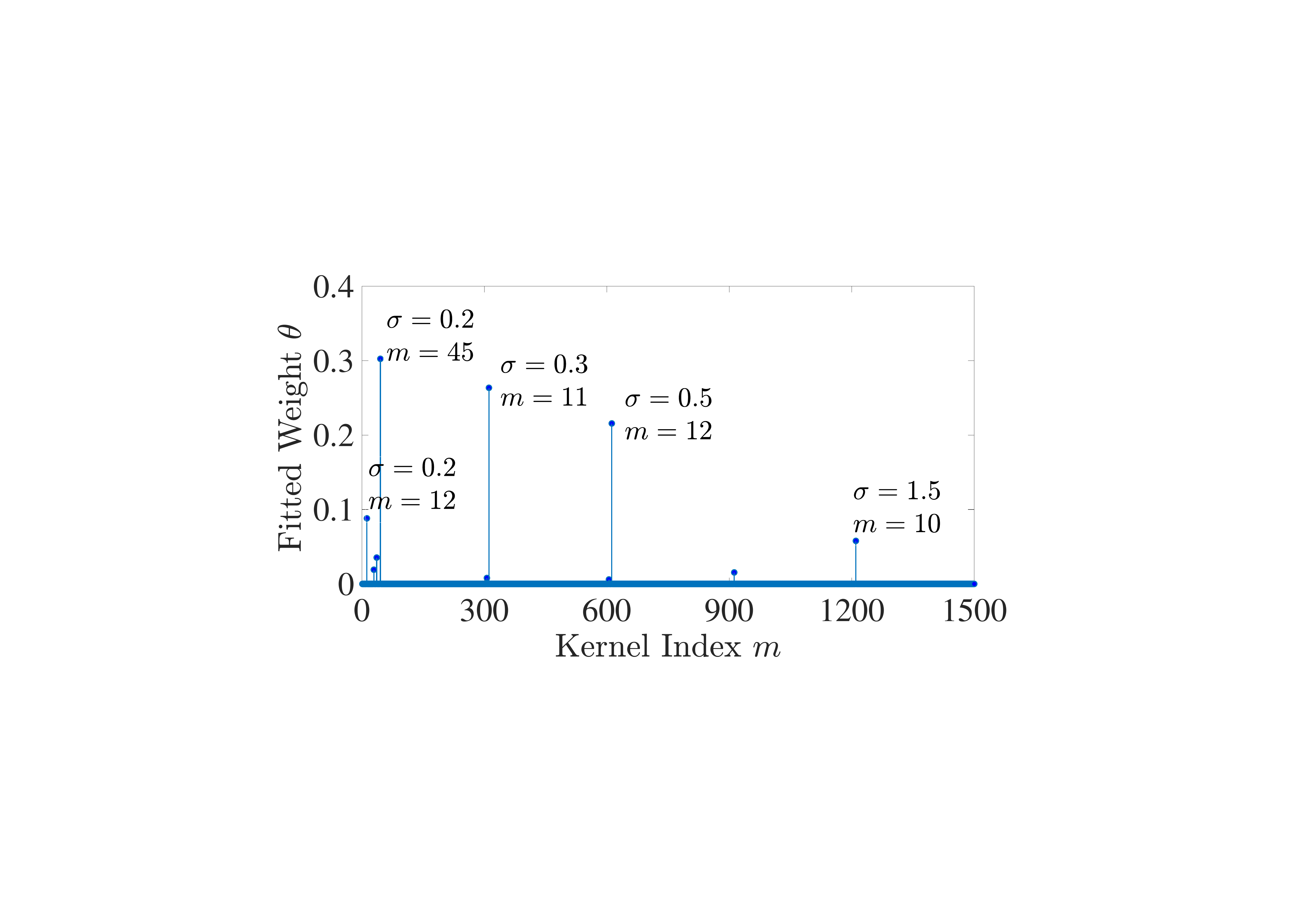
8 . RMSE 0.008. ( ) 5 ML ( 84 ℓ₂−). . ML t = 11 t = 45. ℓ₂ . 9 I-80.

7.4

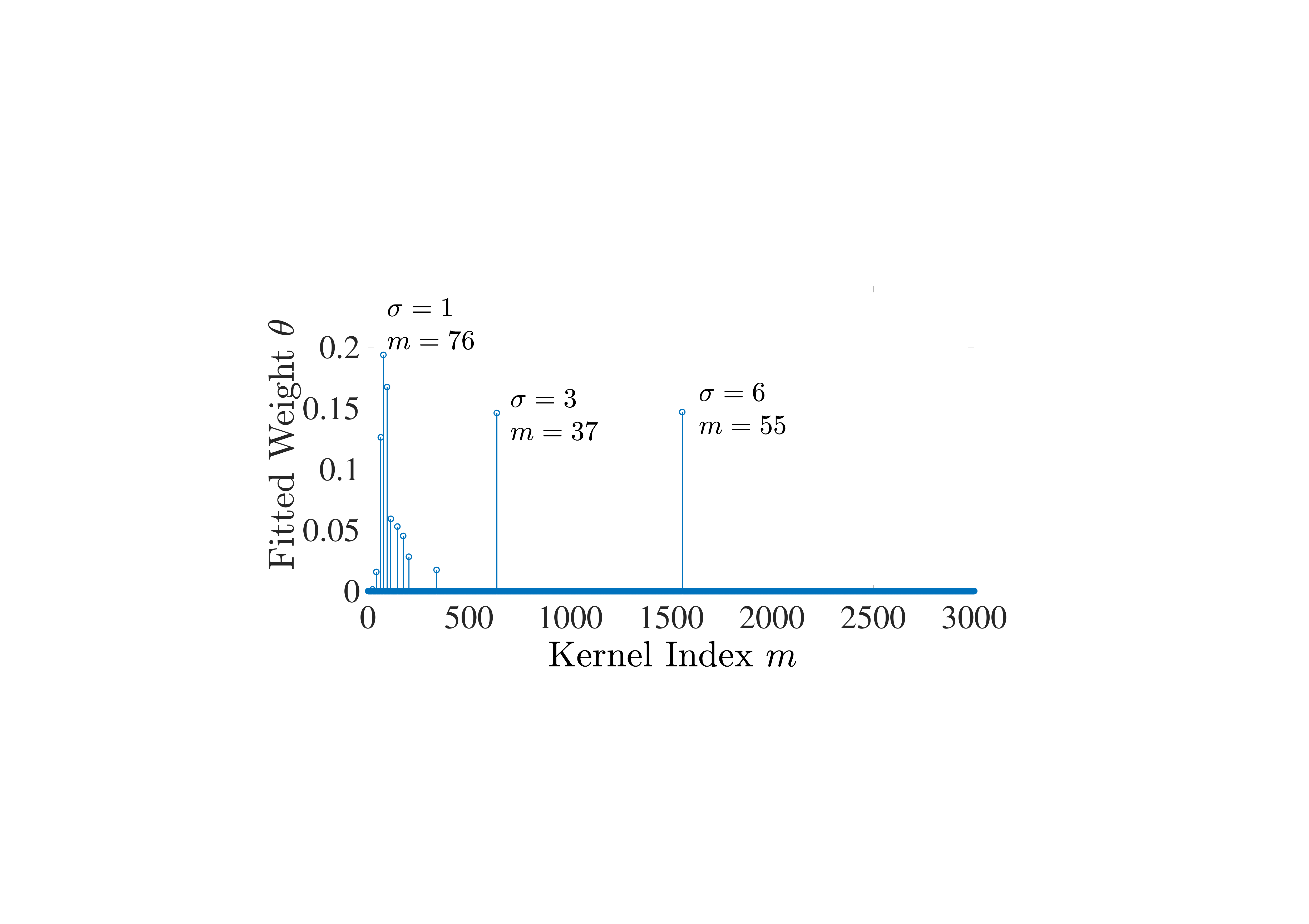
ML ( s) . . ML s_m ∈{1, 2, 3, 4, 5} s= 1. 10 () 10 () M = 1500 ( M′= 300 ) ML M = 300 .

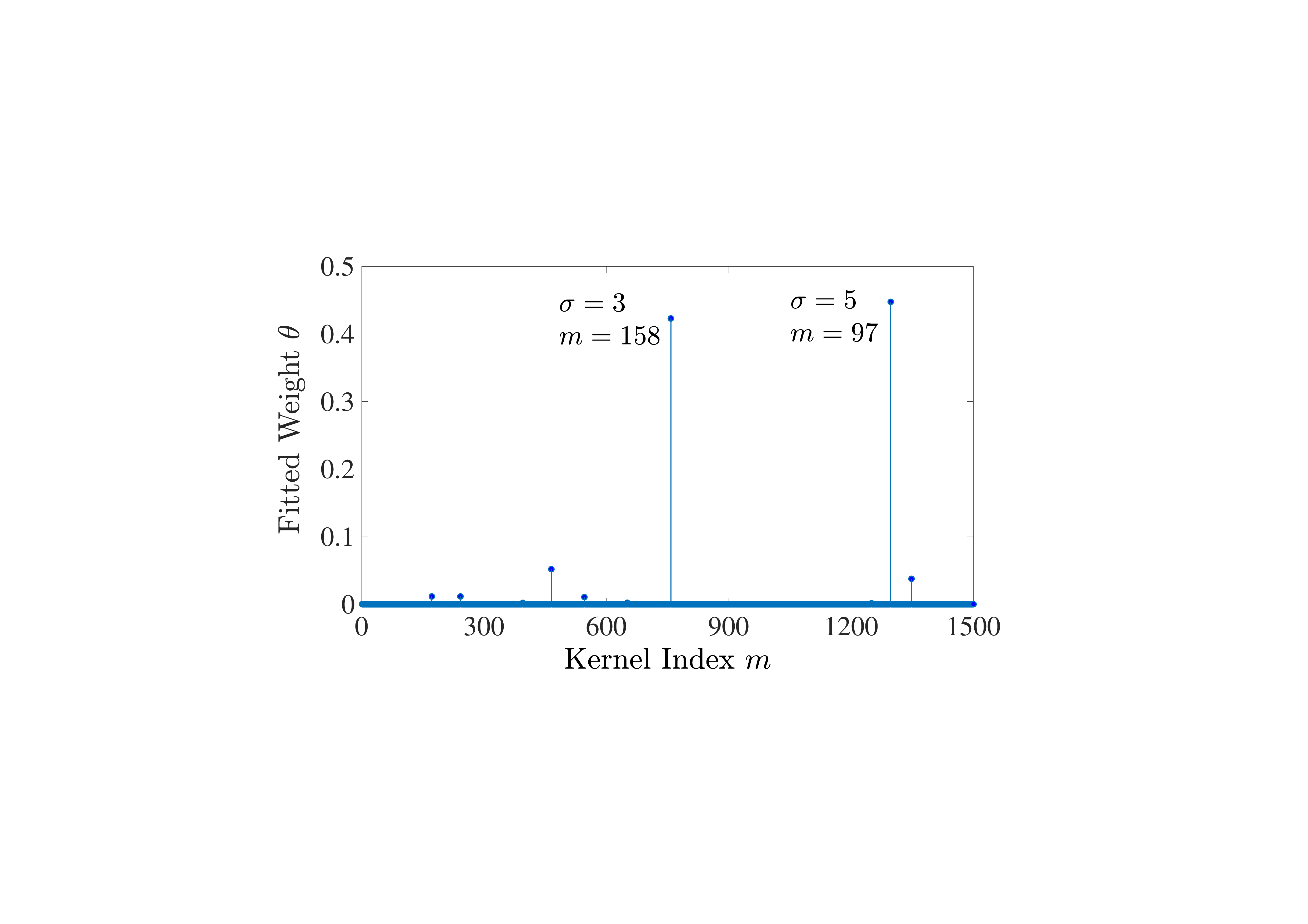
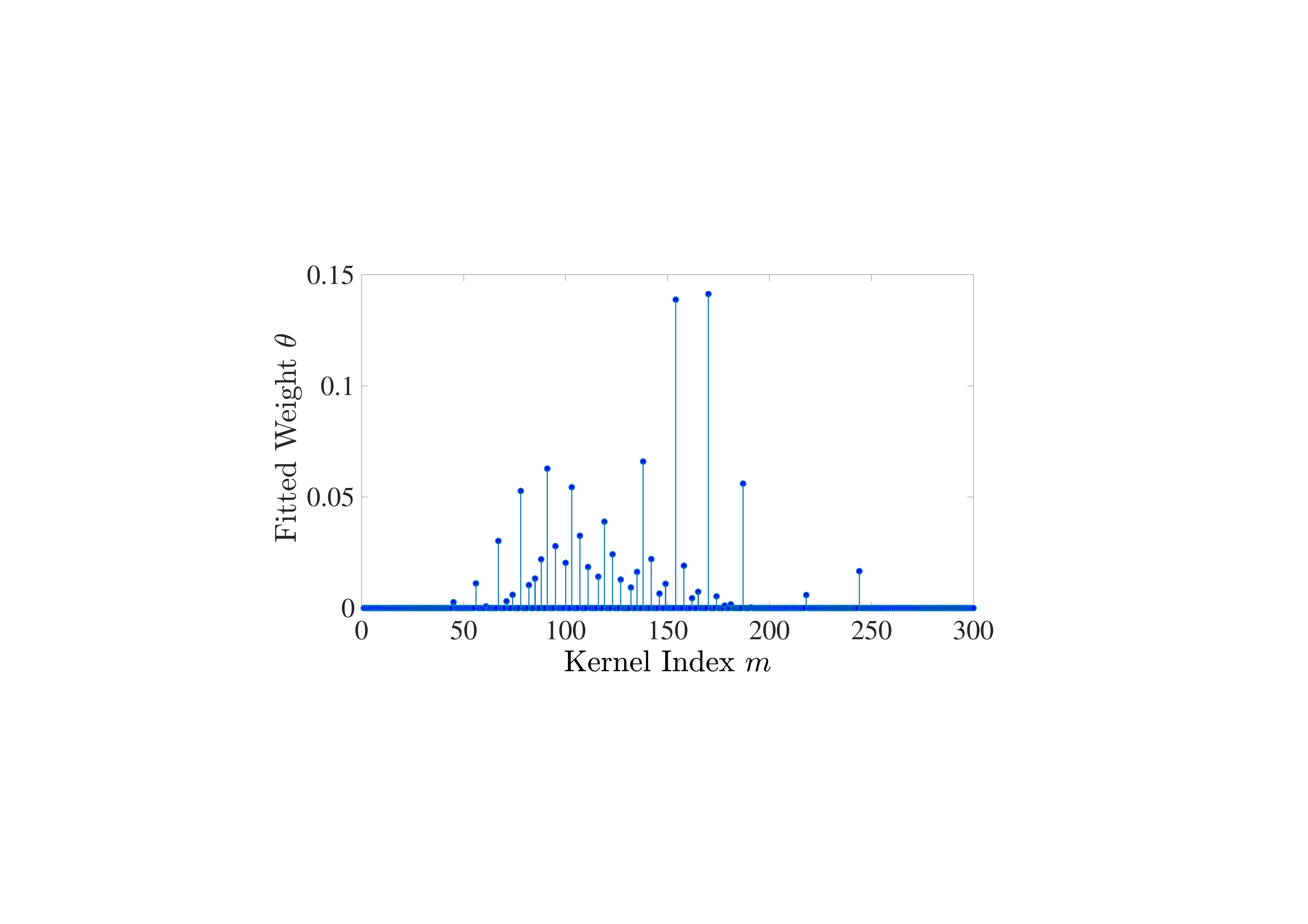
( ). . s= 5 2 11 () ML PW 11 ().

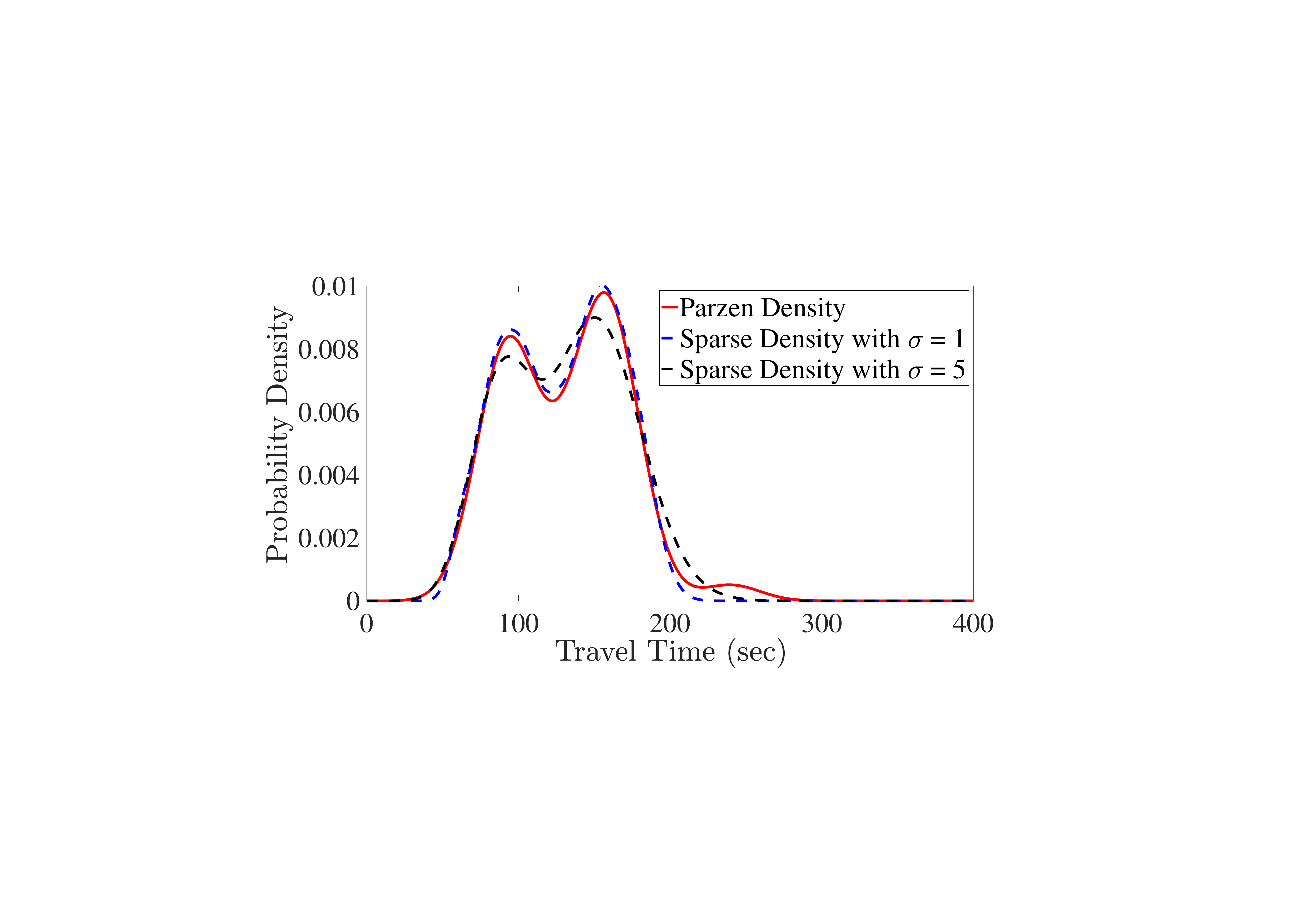
. ML 10 () ML s= 5 t = 97 s= 3 t = 158. () .

7.5

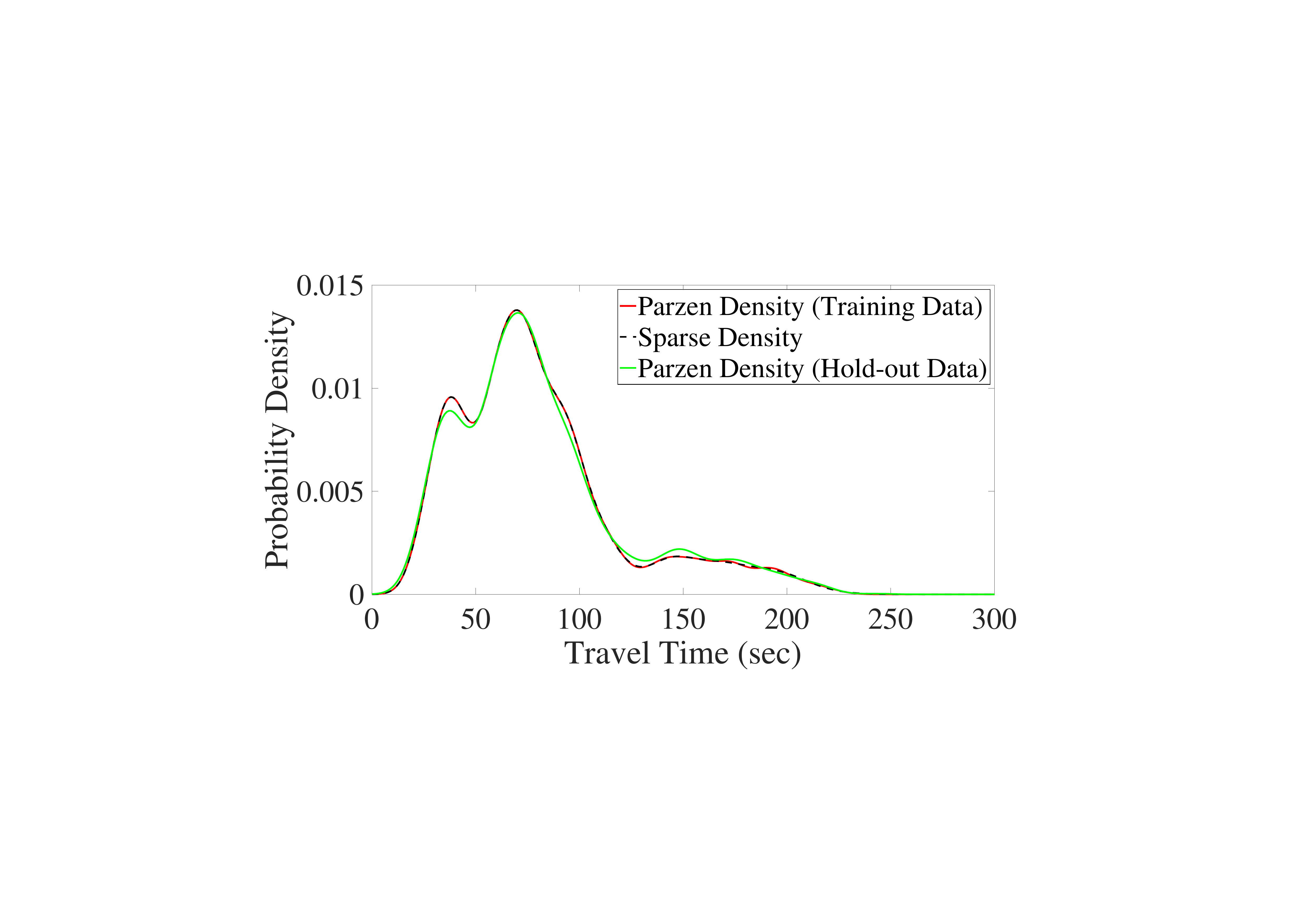
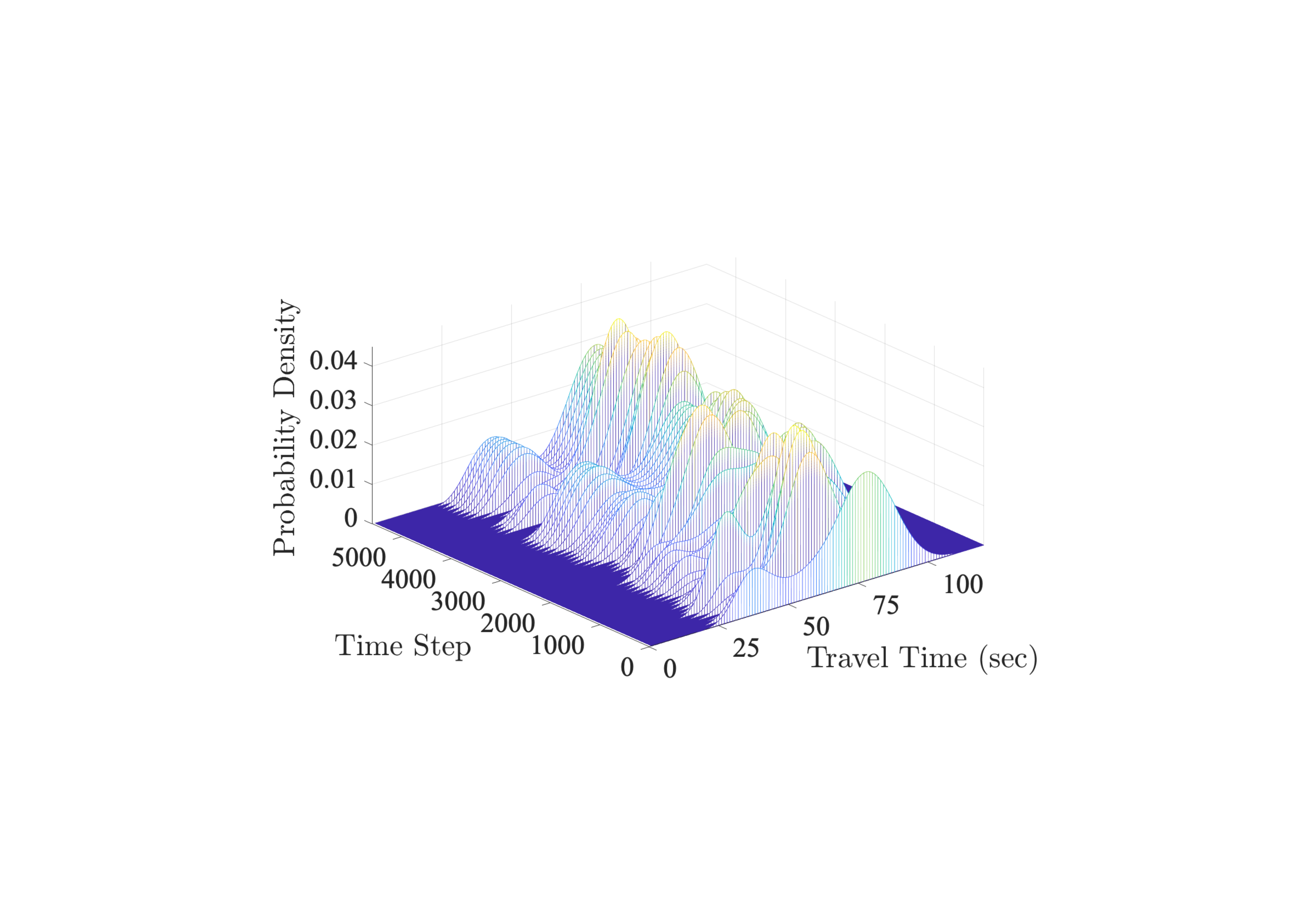
I-80. I-80 W = 100 ( M′= 300, N = 600 s_m ∈{1, 2, 3, 4, 5} M = 1500 ML). ( ) 6.2. PM 12 .

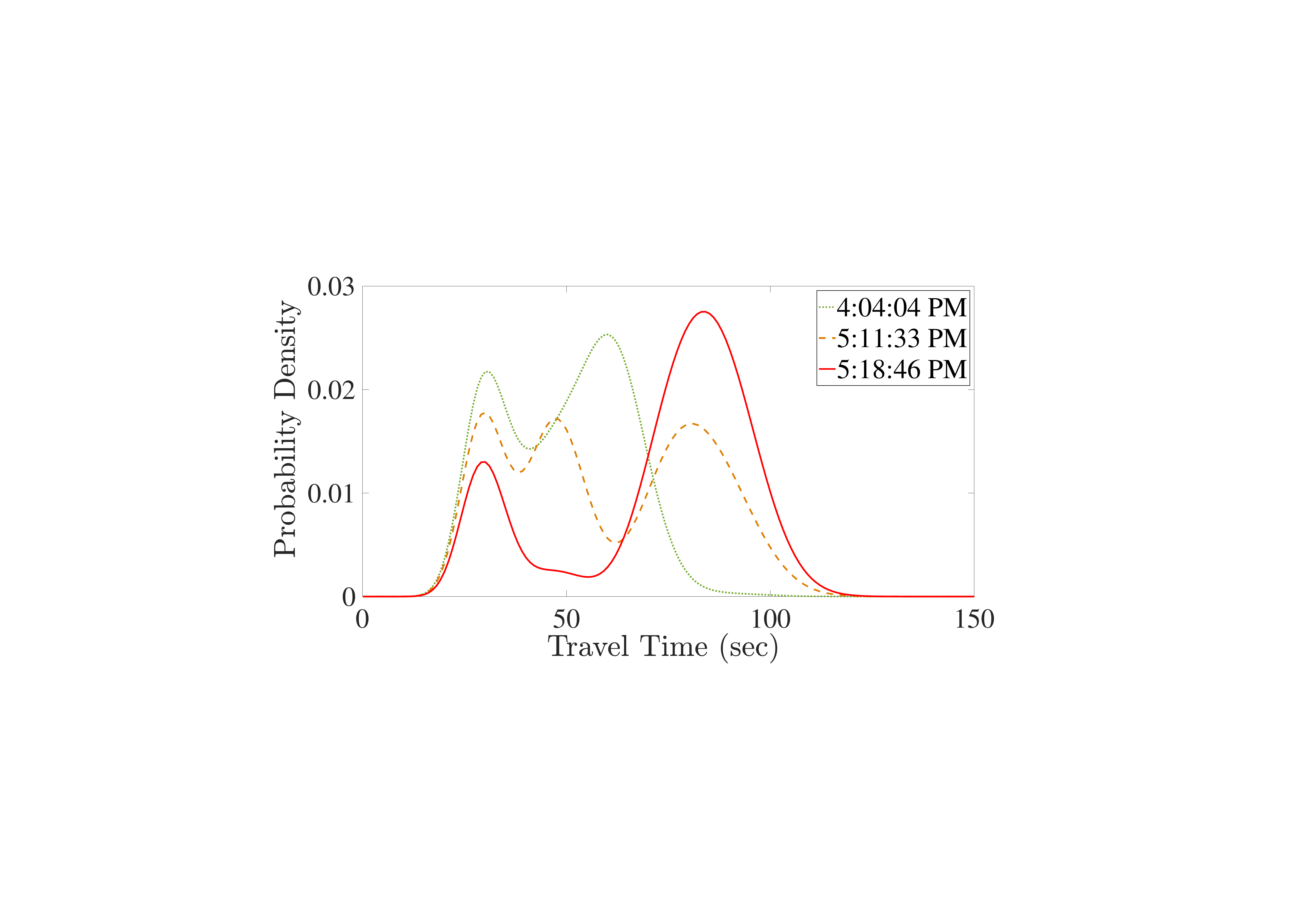
() 4: 04 PM . 80. 5: 08 PM ( ) 3 70 120 . 2 . . .

2.5 2.5 ( ). ( 2.5 45). 13.

8

. . (1) (2) ( ) (3) .

( ) . Mittag-Leffler .

. : (1) (2) . .

. (NSF) CCF-1717207.

A

General
Z₊, R₊	The non-negative integers and non-negative real numbers, respectively
i	The imaginary unit, i ≡ $√ --- − 1$
1_{conditon}	The indicator function, maps to 1 if conditon is true and maps to 0 otherwise
B	The Beta function
G	The Gamma function
E_n	Mittag-Leffler function with parameter n, E_n (t) = _n=0 $--tn-- G(1+nn)$
∥⋅∥	Norm, e.g., ∥y∥₂ is the L₂ norm of y

Traffic-Flow
C(x)	Vehicle crossing time at position x
P(x)	Macroscopic pace at position x
r	Traffic density
V	Equilibrium speed function
Q	Equilibrium flux function (fundamental diagram), Q(r) = rV(r)
P	Equilibrium pace function, which maps traffic density to pace, P(r) = 1/V(r)
r_jam	Jammed traffic density, V(r_jam) = 0
v_fr	Free-flow speed, V(0) = v_fr
v_b	Backward wave speed, $d- dr$ Q(r_jam) = v_b

Probabilities and Related Notions
E	The expectation operator
$( m ) k1 ... kj$	The multinomial coefficient, $( m ) k1 ... kj$ ≡ $--m!-- k1!⋅...⋅kj!$
f _X	The probability density function (PDF) associated with continuous random variable X
p_X	The probability mass function (PMF) associated with discrete random variable X
j_X	The characteristic function associated with random variable X, j_X(s) ≡ Ee^isX
f (y; m)	A PDF evaluated at y with parameter (vector) m. We casually write f (y) ignoring the argument m, so as to lighten notation.
p(y; m)	A PMF evaluated at y with parameter (vector) m. We casually write p(y) ignoring the argument m, so as to lighten notation.
f _G	The PDF of a Gamma distributed random variable
f _M−L	Mittag-Leffler PDF, f _M−L(t; b, s, b) = $--1- sG(b)$ $($ $t s$ $)$ ^b−1 $[$ E_n $($ $($ $t s$ $)$ ^c $)$ $]$ ⁻¹
f _r	The PDF of traffic density
f _P	The PDF of pace
f _T	The PDF of travel time
j_P	The characteristic function of pace
j_G	The characteristic function of a Gamma distributed random variable

Travel Time Data, Empirical Distributions, and Estimated Distributions
w	Regularization parameter
T₁, …, T_S	A sample of S travel times
T_W^(j)	The jth window taken from stream travel time data, T_W^(j) = {T_j, …, T_j+W−1}, where W is the window width
D	Time discretization constant
{t_n}_n=0^N−1	A set of discrete travel times, defining the support (or domain) of the PMFs, t_n = nD
{t_m}_m=0^M−1	A subset of {t_n}_n=0^N−1 representing the locations of the mixture PDFs
t	A function that maps a continuous travel time t to a discrete travel t_n (t_n is the representative of t in the discrete set)
$^f$	Empirical distribution of travel times, also known as the Parzen Window (PW) estimator. $^f$ (t) is the frequency of travel time t ∈R₊, as established empirically.
k_h	A kernel, window, or bin of width h; k_h(t − T_j) provides a measure of the distance between travel time t ∈R₊ and the data point T_j.
f	Mixture PDF (to be estimated)
f_m	The m mixture component of f (a PDF)
q_m	The weight associated with the mth mixture component
q	M dimensional vector of mixture weights
$^p$	Discrete empirical distribution, an N dimensional vector $^p$ = [ $^p$ ₀ … $p^$ _N−1]^⊤ with $^p$ _n $^ f$ (t_n)
p	Discrete mixture distribution, an N dimensional vector p = [p₀ … p_N−1]^⊤ with p_n f (t_n)
c_n	Discretization constant used to define the discrete component densities; specifically, f_n,m ≡ c_nf_m(t_n)
F	The matrix [f_n,m] ∈R₊^N×M: we have p = Fq
Y	A N × N matrix with elements Y_n,i = k_h(t_n −t_i)
$^f$ ^(K)	Parzen density established using the fist K travel times {T₁, …, T_K}
$^f$ ^(j)	Parzen density established using travel time data T_W^(j)
$^p$ ^(K)	Discrete empirical distribution established using the fist K travel times {T₁, …, T_K}
$^p$ ^(j)	Discrete empirical distribution established using travel time data T_W^(j)
$^q$ ^(K)	Estimated mixture weights using the first K travel times {T₁, …, T_K}
$^ q$ ^(j)	Estimated mixture weights using travel time data T_W^(j)

B

[q₀^∗…q_M−1^∗]^⊤ (34) ( ) f_n,m (45). _m=0^M−1q_m^∗ < 1

y_n(t^′, s^′) ≡s^′ f _M
−L $($ t^′; 1 + $tn s′$ , s^′ $)$ ,

(65)

n = 0, 1, …N − 1. t^′s^′

$max n∈ {0,...,N− 1}$ y_n(t^′, s^′) ≤#,

(66)

# > 0. D^′≡ $Ds′$ y_n(t^′, s^′) = s^′ f _M−L(t^′; 1 + nD^′, s^′). t^′s^′ $′ ts′$ = 1

$max n∈{0,...,N −1}$ s^′ f _M
−L(t^′; 1 + nD^′, s^′) = $max n∈{0,...,N−1}$ $1 G(1-+-nD′)E-′(1) D$ .

(67)

R₊ G(x_min) = 0.885603 ( x_min = 1.461632).

$max n∈ {0,...,N− 1}$ y_n(t^′, s^′) ≤ $----1----- 0.88ED ′(1)$

(68)

s^′

E(1) ≥ $-1--- 0.88#$ .

(69)

y(t^′, s^′) F ( ) q= [q^∗⊤, 1 − _m=0^M−1q_m^∗]^⊤. s^′ q^∗ ( D). . q_M = 1 − _n=0^M−1q_m^∗ < 1 y(t^′, s^′) p # ( {t_n}_n=0^N−1 #). LASSO ( ).

C

q . S∈R^M×M S_m,m = s_m :

1 2 − 1 miniq∈mWize 2∥^p − Fq ∥2 + w ∥S q∥1.

(70)

. ( ) . .

W= R₊^M LASSO

1- 2 ⊤ −1 miqn∈iRmMi+z1e 2∥ ^p− Fq ∥2 + w1 S q, +

(71)

z- 2 M 1-- M minqi∈mRiMz+e1 2 ∥^p− Fq∥2 + zw smqm − log (qi). m=0 m=0

(72)

D

LASSO (52) . "" q . q |q_i| < e∥q∥ e . e= 10⁻³. supp ( $^ q$ ) ( ) s_w ≡|supp(q)|. () . : F_s ∈R^N×s_w F $^q$ _s :

2 minqis∈mWisze ∥^p− Fsqs ∥2.

(73)

W_s = R₊^s_w.

E

w . w ( ). ( ). w ( ) ( ) : ( ) . w . . w k [Efron and Gong, 1983, Turney, 1994]. . LASSO.

w . [Reid et al., 2013, Sun and Zhang, 2012] LASSO

2 S2w ≡ ∥-^p−-Fq-(w)∥2, M − sw

(74)

s_w ≡|supp(q(w))| ( D) . q(w) LASSO () w. S_w² (74) (i) ℓ₂− ∥ $^p$ −Fq(w)∥₂² (ii) (M − s_w) ( q): . . S_w² s_w < M w 0 s_w = M (S_w² (w_min, +) w_min > 0 q w) ( ).

w = 0 :

minimize ∥p^− Fq ∥22, q∈W

(75)

ℓ₂− ( ) (s_w = M ). w > w₀

w ≡ ∥F ⊤^p∥ , 0

(76)

(s_w = 0) ℓ₂− ∥ $^p$ ∥₂². w S_w². w : w₀ S_w² w_k = h^kw₀ h∈(0, 1) h= 0.95 k . :

$∥ ^p− Fq (w )∥ − ∥^p− Fq(w )∥ ----------k+1--2-------------k--2 ∥ ^p− Fq (wk)∥2$ < e′,

(77)

e′= 10⁻³. . ( 6 ).

References

R. Abbi, E. El-Darzi, C. Vasilakis, and P. Millard. Analysis of stopping criteria for the EM algorithm in the context of patient grouping according to length of stay. In 4th International IEEE Conference on Intelligent Systems (IS’08), pages 3–9, 2008.

M. Afonso, J. Bioucas-Dias, and M. Figueiredo. Fast image recovery using variable splitting and constrained optimization. IEEE Transactions on Image Processing, 19(9): 2345–2356, 2010.

H. Al-Deek and E. Emam. New methodology for estimating reliability in transportation networks with degraded link capacities. Journal of Intelligent Transportation Systems, 10(3):117–129, 2006.

C. Archambeau, J. Lee, and M. Verleysen. On convergence problems of the EM Algorithm for Finite Gaussian Mixtures. In European Symposium on Artificial Neural Networks, pages 99–106, 2003.

M. Arezoumandi. Estimation of travel time reliability for freeways using mean and standard deviation of travel time. Journal of Transportation Systems Engineering and Information Technology, 11 (6):74–84, 2011.

A. Beck and M. Teboulle. A fast iterative shrinkage-thresholding algorithm for linear inverse problems. SIAM Journal on Imaging Sciences, 2(1):183–202, 2009.

C. Biernacki, G. Celeux, and G. Govaert. Choosing starting values for the EM algorithm for getting the highest likelihood in multivariate Gaussian mixture models. Computational Statistics & Data Analysis, 41(3):561–575, 2003.

C. Bishop. Pattern recognition and machine learning. Springer, New York, 2006.

S. Boyd and L. Vandenberghe. Convex optimization. Cambridge University Press, Cambridge, UK, 2004.

T. Cacoullos. Estimation of a multivariate density. Annals of the Institute of Statistical Mathematics, 18(1):179–189, 1966.

Malachy Carey and YE Ge. Alternative conditions for a well-behaved travel time model. Transportation Science, 39(3):417–428, 2005a.

Malachy Carey and YE Ge. Convergence of a discretised travel-time model. Transportation Science, 39(1):25–38, 2005b.

S. Chakraborty and S. Ong. Mittag-Leffler function distribution – A new generalization of hyper-Poisson distribution. Journal of Statistical Distributions and Applications, 4(8):1–17, 2017.

P. Chen, K. Yin, and J. Sun. Application of finite mixture of regression model with varying mixing probabilities to estimation of urban arterial travel times. Transportation Research Record: Journal of the Transportation Research Board, 2442:96–105, 2014.

S. Chen. Probability density function estimation using Gamma kernels. Annals of the Institute of Statistical Mathematics, 52(3):471–480, 2000.

S. Chen, X. Hong, and C. Harris. Sparse kernel density construction using orthogonal forward regression with leave-one-out test score and local regularization. IEEE Transactions on Systems, Man, and Cybernetics Part B, 34(4):1708–1717, 2004.

S. Chen, X. Hong, and C. Harris. An orthogonal forward regression technique for sparse kernel density estimation. Neurocomputing, 71(4):931–943, 2008.

J. Del Castillo and F. Benitez. On the functional form of the speed-density relationship. i: General theory, ii: Empirical investigation. Transportation Research Part B, 29(5):373–406, 1995.

D. Dilip, N. Freris, and Saif Jabari. Sparse estimation of travel time distributions using Gamma kernels, paper no. 17-02971. In 96th Annual Meeting of the Transportation Research Board, 2017.

L. Du, S. Peeta, and Y. Kim. An adaptive information fusion model to predict the short-term link travel time distribution in dynamic traffic networks. Transportation Research Part B, 46(1):235–252, 2012.

B. Efron and G. Gong. A leisurely look at the bootstrap, the jackknife, and cross-validation. The American Statistician, 37(1):36–48, 1983.

E. Emam and H. Al-Deek. Using real-life dual-loop detector data to develop new methodology for estimating freeway travel time reliability. Transportation Research Record: Journal of the Transportation Research Board, 1959:140–150, 2006.

Y. Feng, J. Hourdos, and G. Davis. Probe vehicle based real-time traffic monitoring on urban roadways. Transportation Research Part C, 40:160–178, 2014.

M. Fosgerau and D. Fukuda. Valuing travel time variability: Characteristics of the travel time distribution on an urban road. Transportation Research Part C, 24:83–101, 2012.

R. Franklin. The structure of a traffic shock wave. Civil Engineering and Public Works Review, 56:1186–1188, 1961.

N. Freris, O. Öçal, and M. Vetterli. Recursive compressed sensing. arXiv preprint:1312.4895, 2013a.

N. Freris, O. Öçal, and M. Vetterli. Compressed Sensing of Streaming data. In Proceedings of the 51st Allerton Conference on Communication, Control and Computing, pages 1242–1249, 2013b.

Gianpaolo Ghiani and Emanuela Guerriero. A note on the Ichoua, Gendreau, and Potvin (2003) travel time model. Transportation Science, 48(3):458–462, 2014.

Andrés Gómez, Ricardo Mariño, Raha Akhavan-Tabatabaei, Andrés L Medaglia, and Jorge E Mendoza. On modeling stochastic travel and service times in vehicle routing. Transportation Science, 50(2):627–641, 2016.

M. Grant and S. Boyd. CVX: Matlab software for disciplined convex programming, version 2.1. http://cvxr.com/cvx, March 2014.

F. Guo, H. Rakha, and S. Park. Multistate model for travel time reliability. Transportation Research Record: Journal of the Transportation Research Board, 2188:46–54, 2010.

F. Haight. Mathematical theories of traffic flow. Academic Press, New York, 1963.

H. Haubold, A. Mathai, and R. Saxena. Mittag-Leffler functions and their applications. Journal of Applied Mathematics, 2011, 2011.

A. Hofleitner, R. Herring, and A. Bayen. Arterial travel time forecast with streaming data: A hybrid approach of flow modeling and machine learning. Transportation Research Part B, 46(9):1097–1122, 2012a.

A. Hofleitner, R. Herring, and A. Bayen. Probability distributions of travel times on arterial networks: A traffic flow and horizontal queuing theory approach, paper no. 12-0798. In 91st Annual Meeting of the Transportation Research Board, 2012b.

A. Hofleitner, T. Rabbani, L. El Ghaoui, and A. Bayen. Online Homotopy Algorithm for a Generalization of the LASSO. IEEE Transactions on Automatic Control, 58(12):3175–3179, 2013.

A. Hofleitner, T. Rabbani, M. Rafiee, L. El Ghaoui, and A. Bayen. Learning and estimation applications of an online homotopy algorithm for a generalization of the LASSO. Discrete and Continuous Dynamical Systems, 7(3):503–523, 2014.

T. Hunter, T. Das, M. Zaharia, P. Abbeel, and A. Bayen. Large-scale estimation in cyberphysical systems using streaming data: A case study with arterial traffic estimation. IEEE Transactions on Automation Science and Engineering, 10(4):884–898, 2013.

Soumia Ichoua, Michel Gendreau, and Jean-Yves Potvin. Vehicle dispatching with time-dependent travel times. European journal of operational research, 144(2):379–396, 2003.

S.E. Jabari, J. Zheng, and H. Liu. A probabilistic stationary speed–density relation based on Newells simplified car-following model. Transportation Research Part B, 68: 205–223, 2014.

S.E. Jabari, F. Zheng, H. Liu, and M. Filipovska. Stochastic Lagrangian modeling of traffic dynamics, paper no. 18-04170. In 97th Annual Meeting of the Transportation Research Board, 2018.

E. Jenelius and H. Koutsopoulos. Travel time estimation for urban road networks using low frequency probe vehicle data. Transportation Research Part B, 53:64–81, 2013.

E. Jenelius and H. Koutsopoulos. Probe vehicle data sampled by time or space: consistent travel time allocation and estimation. Transportation Research Part B, 71: 120–137, 2015.

Y. Ji and H.M. Zhang. Travel time distributions on urban streets: Estimation with hierarchical Bayesian mixture model and application to traffic analysis with high-resolution bus probe data, paper no. 13-4377. In 92nd Annual Meeting of the Transportation Research Board, 2013.

D. Karlis and E. Xekalaki. Choosing initial values for the EM algorithm for finite mixtures. Computational Statistics & Data Analysis, 41(3):577–590, 2003.

E. Kazagli and H. Koutsopoulos. Arterial travel time estimation from automatic number plate recognition data. Transportation Research Record: Journal of the Transportation Research Board, 2391:22–31, 2013.

Jeffrey P Kharoufeh and Natarajan Gautam. Deriving link travel-time distributions via stochastic speed processes. Transportation Science, 38(1):97–106, 2004.

J. Kim and H. Mahmassani. A finite mixture model of vehicle-to-vehicle and day-to-day variability of traffic network travel times. Transportation Research Part C, 46: 83–97, 2014.

J. Kim and H. Mahmassani. Compound Gamma representation for modeling travel time variability in a traffic network. Transportation Research Part B, 80:40–63, 2015.

S. Kim, K. Koh, M. Lustig, S. Boyd, and D. Gorinevsky. An interior-point method for large-scale-regularized least squares. IEEE Journal of Selected Topics in Signal Processing, 1(4):606–617, 2007.

C. Lacour, P. Massart, and V. Rivoirard. Estimator selection: A new method with applications to kernel density estimation. arXiv preprint arXiv:1607.05091, 2016.

M. Lighthill and G. Whitham. On kinematic waves. i: Flood movement in long rivers, ii: A theory of traffic flow on long crowded roads. In Proceedings of the Royal Society (London) A229, pages 281–345, 1955.

W. Lin, Y. Wang, Y. Zhuang, and S. Zhang. Evaluate the number of clusters in finite mixture models with the penalized histogram difference criterion. Journal of Process Control, 23(8):1052–1062, 2013.

S. Mukherjee and V. Vapnik. Support vector method for multivariate density estimation (AI Memo 1653), 1999. URL ftp://publications.ai.mit.edu/ai-publications/1500-1999/AIM-1653.ps.

Y. Nesterov. Gradient methods for minimizing composite functions. Mathematical Programming, 140(1):125–161, 2013.

G. Newell. Nonlinear effects in the dynamics of car following. Operations Research, 9 (2):209–229, 1961.

N. Parikh and S. Boyd. Proximal Algorithms. Foundations and Trends in Optimization, 1(3):127–239, 2014.

E. Parzen. On estimation of a probability density function and mode. The Annals of Mathematical Statistics, 33(3):1065–1076, 1962.

A. Polus. A study of travel time and reliability on arterial routes. Transportation, 8(2): 141–151, 1979.

W. Pu. Analytic relationships between travel time reliability measures. Transportation Research Record: Journal of the Transportation Research Board, 2254:122–130, 2011.

V. Punzo, M. Borzacchiello, and B. Ciuffo. On the assessment of vehicle trajectory data accuracy and application to the Next Generation SIMulation (NGSIM) program data. Transportation Research Part C, 19(6):1243–1262, 2011.

M. Rahmani, E. Jenelius, and H. N Koutsopoulos. Non-parametric estimation of route travel time distributions from low-frequency floating car data. Transportation Research Part C, 58:343–362, 2015.

H. Rakha, I. El-Shawarby, Arafeh M., and F. Dion. Estimating path travel-time reliability. In Proceeding of the 2006 IEEE Conference on Intelligent Transportation Systems, pages 236–241, 2006.

H. A Rakha, J. Du, S. Park, F. Guo, Z. Doerzaph, D. Viita, G. Golembiewski, B. Katz, N. Kehoe, and H.. Rigdon. Feasibility of using in-vehicle video data to explore how to modify driver behavior that causes nonrecurring congestion (SHRP 2 Report S2-L10-RR-01). Transportation Research Board, Washington, D.C., 2011.

M. Ramezani and N. Geroliminis. On the estimation of arterial route travel time distribution with Markov chains. Transportation Research Part B, 46(10):1576–1590, 2012.

M. Ramezani and N. Geroliminis. Queue profile estimation in congested urban networks with probe data. Computer-Aided Civil and Infrastructure Engineering, 30(6): 414–432, 2015.

Š. Raudys. On the effectiveness of Parzen window classifier. Informatica, 2(2):434–454, 1991.

R. Redner and H. Walker. Mixture densities, maximum likelihood and the EM algorithm. SIAM Review, 26(2):195–239, 1984.

S. Reid, R. Tibshirani, and J. Friedman. A study of error variance estimation in LASSO regression. arXiv preprint arXiv:1311.5274, 2013.

P. Richards. Shock waves on the highway. Operations Research, 4(1):42–51, 1956.

A. Richardson and M. Taylor. Travel time variability on commuter journeys. High Speed Ground Transportation Journal, 12(1), 1978.

B. Silverman. Density estimation for statistics and data analysis, volume 26. CRC Press, Boca Raton, FL, 1986.

P. Sopasakis, N. Freris, and P. Patrinos. Accelerated reconstruction of a compressively sampled data stream. In 24th IEEE European Signal Processing Conference (EUSIPCO), pages 1078–1082, 2016.

T. Sun and C. Zhang. Scaled sparse linear regression. Biometrika, pages 1–20, 2012.

M. Taylor. Fosgerau’s travel time reliability ratio and the Burr distribution. Transportation Research Part B, 97:50–63, 2017.

Robert Tibshirani. Regression shrinkage and selection via the lasso. Journal of the Royal Statistical Society. Series B, pages 267–288, 1996.

P. Turney. A theory of cross-validation error. Journal of Experimental and Theoretical Artificial Intelligence, 6(4):361–391, 1994.

N. Wan, G. Gomes, A. Vahidi, and R. Horowitz. Prediction on travel-time distribution for freeways using online expectation maximization algorithm, paper no. 14-3221. In 93rd Annual Meeting of the Transportation Research Board, 2014.

S. Wright, R. Nowak, and M. Figueiredo. Sparse reconstruction by separable approximation. IEEE Transactions on Signal Processing, 57(7):2479–2493, 2009.

C. Wu. On the convergence properties of the EM algorithm. The Annals of Statistics, pages 95–103, 1983.

X. Xu, A. Chen, L. Cheng, and H. Lo. Modeling distribution tail in network performance assessment: A mean-excess total travel time risk measure and analytical estimation method. Transportation Research Part B, 66:32–49, 2014.

F. Yang, M. Yun, and X. Yang. Travel time distribution under interrupted flow and application to travel time reliability. Transportation Research Record: Journal of the Transportation Research Board, 2466:114–124, 2014.

F. Zheng, S.E. Jabari, H. Liu, and D. Lin. Traffic state estimation using stochastic Lagrangian dynamics. Transportation Research Part B, 115:143–165, 2018.

Fangfang Zheng, Henk Van Zuylen, and Xiaobo Liu. A methodological framework of travel time distribution estimation for urban signalized arterial roads. Transportation Science, 51(3):893–917, 2017.